Wolfram Function Repository
Instant-use add-on functions for the Wolfram Language
Function Repository Resource:
Create a fast Fourier transform calculation in graphical form
ResourceFunction["FastFourierGraph"][dim] returns an edge-weighted, time-ordered multiway graph on 2dim×2dim vertices, which describes the fast Fourier transform of a length 2dim vector. | |
ResourceFunction["FastFourierGraph"][data] takes a list of data with length 2dim and adds it to the graph under the annotation key VertexWeight. |
Calculate the graph for the base case of the fast Fourier transform:
| In[1]:= |
| Out[1]= |  |
Plot the next induced case:
| In[2]:= |
| Out[2]= | 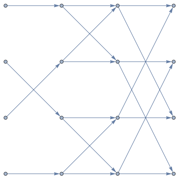 |
Color edges according to phases:
| In[3]:= | ![Graph[graph, EdgeStyle -> MapThread[
#1 -> Darker[Hue[1/10 + (9/10) (1/2) Mod[Arg[#2]/Pi, 2]]] &,
{EdgeList[graph], AnnotationValue[graph, EdgeWeight]
}]]](https://www.wolframcloud.com/obj/resourcesystem/images/21d/21dbf0fc-45ef-41e5-bf3d-31b2e1fa0502/6b1fed2d6b3a4c7f.png) |
| Out[3]= | 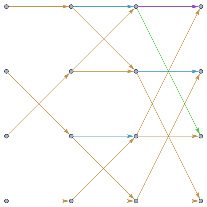 |
Notice n log n complexity in rectangular dimensions of subsequent graphs:
| In[4]:= | ![With[{graph0 = ResourceFunction["FastFourierGraph"][#]},
Graph[graph0, EdgeStyle -> MapThread[# -> Darker[
Hue[1/10 + ((9/10) (1/2)) Mod[Arg[#2]/Pi, 2]]]& , {
EdgeList[graph0], AnnotationValue[graph0, EdgeWeight]}]]] & /@ Range[4]](https://www.wolframcloud.com/obj/resourcesystem/images/21d/21dbf0fc-45ef-41e5-bf3d-31b2e1fa0502/70d8805d277fbc95.png) |
| Out[4]= | 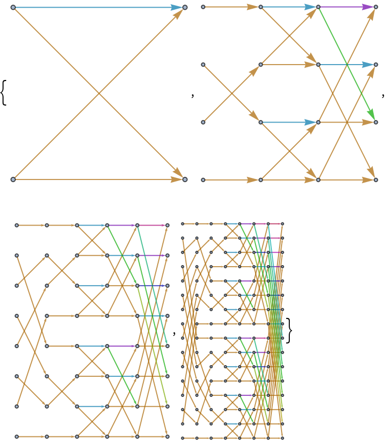 |
Blow up the graphs to see their free-form structure using "SpringElectricalEmbedding":
| In[5]:= | ![With[{graph0 = ResourceFunction["FastFourierGraph"][#]},
Graph[graph0, EdgeStyle -> MapThread[# -> Darker[
Hue[1/10 + ((9/10) (1/2)) Mod[Arg[#2]/Pi, 2]]]& , {
EdgeList[graph0], AnnotationValue[graph0, EdgeWeight]}],
GraphLayout -> "SpringElectricalEmbedding",
VertexCoordinates -> Automatic]] & /@ Range[4]](https://www.wolframcloud.com/obj/resourcesystem/images/21d/21dbf0fc-45ef-41e5-bf3d-31b2e1fa0502/324b9eeab70eb61e.png) |
| Out[5]= | 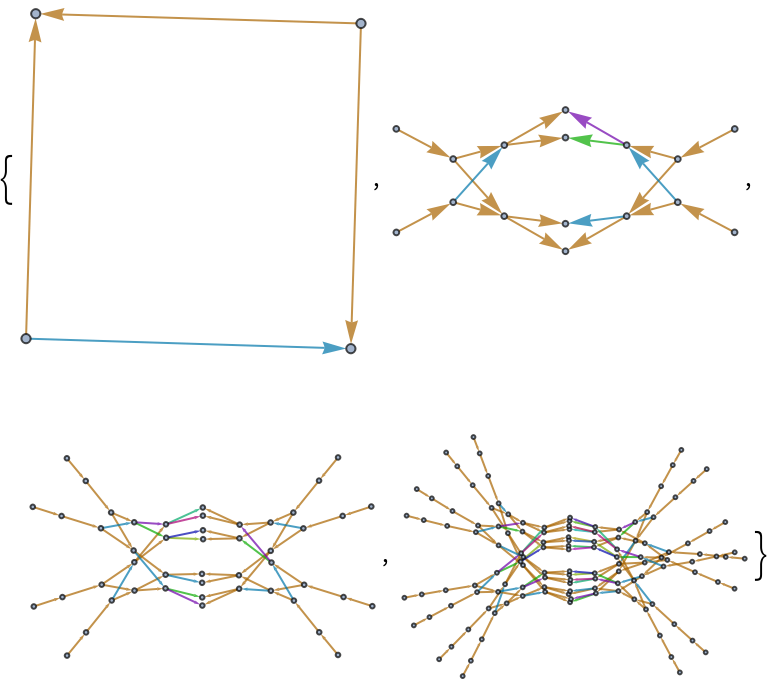 |
Create a graph from data:
| In[6]:= |
| Out[6]= |  |
Use the option "ComputeValues"→True to compute the transformation values while generating the graph:
| In[7]:= |
| Out[7]= |  |
See the fast Fourier transformation values by retrieving the VertexWeight:
| In[8]:= |
| Out[8]= |
Depict results of the calculation as above:
| In[9]:= |
| Out[9]= | 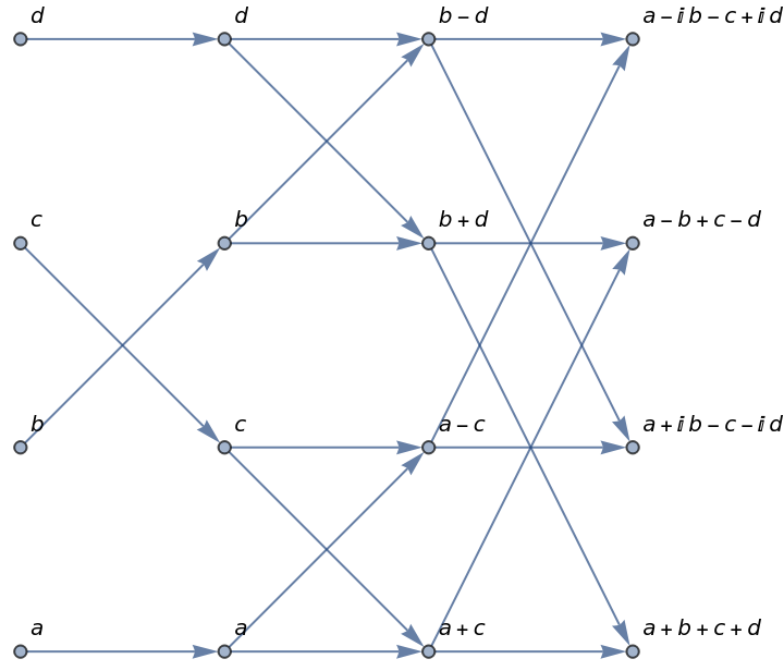 |
Compare with the standard method using FourierMatrix:
| In[10]:= |
| Out[10]= |
Apply a similar validation technique for different input lengths:
| In[11]:= | ![Function[{exp}, ComplexExpand[Subtract[
With[{graph = ResourceFunction["FastFourierGraph"][
c /@ Range[2^exp], "ComputeValues" -> True]},
Part[Sort@Transpose[{VertexList@graph,
AnnotationValue[graph, VertexWeight]}],
-2^exp ;; -1, 2]],
Sqrt[2^exp] Dot[FourierMatrix[2^exp],
(c /@ Range[2^exp])]]]] /@ Range[4]](https://www.wolframcloud.com/obj/resourcesystem/images/21d/21dbf0fc-45ef-41e5-bf3d-31b2e1fa0502/3343e5f34dd654cd.png) |
| Out[11]= |
Input should be a list of length 2n for some integer n>0:
| In[13]:= |
| Out[13]= |
| In[14]:= |
| Out[14]= |
Timing statistics look very slow compared to the built-in Fourier:
| In[15]:= | ![Grid[{{Text@"Evaluation Time"}, {
AbsoluteTiming[Fourier[RandomReal[1, 128]];
][[1]]}}, Spacings -> {1, 1}]](https://www.wolframcloud.com/obj/resourcesystem/images/21d/21dbf0fc-45ef-41e5-bf3d-31b2e1fa0502/5fa98edf8c26b26c.png) |
| Out[15]= |
| In[16]:= | ![Grid[{Text /@ {"Compile Time", "Evaluation Time"},
{#[[1]], #[[2]] - #[[1]]} &@{
AbsoluteTiming[
ResourceFunction["FastFourierGraph"][RandomReal[1, 128]];][[
1]],
AbsoluteTiming[
ResourceFunction["FastFourierGraph"][N@RandomReal[1, 128],
"ComputeValues" -> True];][[1]]}},
Spacings -> {2, 1}]](https://www.wolframcloud.com/obj/resourcesystem/images/21d/21dbf0fc-45ef-41e5-bf3d-31b2e1fa0502/660615a31bd3fd4a.png) |
| Out[16]= |
Compile time is relatively slow compared to ButterflyGraph:
| In[17]:= | ![Grid[Prepend[
SetAccuracy[{AbsoluteTiming[
ResourceFunction["FastFourierGraph"][#]][[1]],
AbsoluteTiming[ButterflyGraph[#]][[1]]}, 6] & /@ Range[5],
{"FastFourierGraph", "ButterflyGraph"}], Spacings -> {2, 0.5},
Alignment -> Center]](https://www.wolframcloud.com/obj/resourcesystem/images/21d/21dbf0fc-45ef-41e5-bf3d-31b2e1fa0502/34ffdf97fd451bb0.png) |
| Out[17]= |  |
Follow the different paths a value can take from input to output:
| In[18]:= | ![Grid[With[{graph = ResourceFunction["FastFourierGraph"][2]},
Outer[Graph[HighlightGraph[graph,
Graph[DirectedEdge @@@ Partition[
First[FindPath[graph, {0, #1}, {3, #2}]], 2, 1]]],
VertexCoordinates -> Automatic,
GraphLayout -> "SpringElectricalEmbedding"] &,
Range[4], Range[4], 1]], Frame -> All, FrameStyle -> LightGray]](https://www.wolframcloud.com/obj/resourcesystem/images/21d/21dbf0fc-45ef-41e5-bf3d-31b2e1fa0502/46f2f10bed1a42f4.png) |
| Out[18]= | 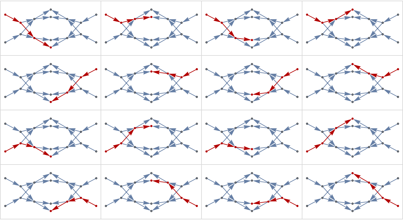 |
Plot an intensity profile:
| In[19]:= | ![With[{data = AnnotationValue[
ResourceFunction["FastFourierGraph"][ReplacePart[Table[0, {64}],
# -> 1 & /@ Range[4]], "ComputeValues" -> True], VertexWeight][[-64 ;; -1]]},
ListPlot[RotateRight[Re[Conjugate[#] #] &@data, 32],
AxesLabel -> {"Position", "Intensity"}]
]](https://www.wolframcloud.com/obj/resourcesystem/images/21d/21dbf0fc-45ef-41e5-bf3d-31b2e1fa0502/1271aba4efe51fa1.png) |
| Out[19]= | 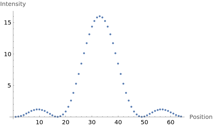 |
This work is licensed under a Creative Commons Attribution 4.0 International License
![IsomorphicGraphQ[ButterflyGraph[#],
UndirectedGraph[VertexDelete[
ResourceFunction["FastFourierGraph"][#], {{x_ /; x < (# - 1), _}}]
]] & /@ Range[5]](https://www.wolframcloud.com/obj/resourcesystem/images/21d/21dbf0fc-45ef-41e5-bf3d-31b2e1fa0502/1808e36a189ec10c.png)