Wolfram Function Repository
Instant-use add-on functions for the Wolfram Language
Function Repository Resource:
Evaluate the boundary curve of the field of values of a matrix
ResourceFunction["MatrixFieldOfValues"][m,t] evaluates the boundary curve of the field of values for a numerical square matrix m at t. |
Compute a point on the boundary curve of the field of values for a matrix:
| In[1]:= |
| Out[1]= |
A square matrix:
| In[2]:= |
Visualize the field of values of the matrix along with its eigenvalues:
| In[3]:= | ![Show[ParametricPlot[
ReIm[ResourceFunction["MatrixFieldOfValues"][mat, t]], {t, 0, 2 \[Pi]}, Axes -> None, Frame -> True],
ComplexListPlot[Eigenvalues[N[mat]], PlotMarkers -> {"+", Large}, PlotStyle -> ColorData[97, 4]]]](https://www.wolframcloud.com/obj/resourcesystem/images/1fe/1fe15e26-4cd0-4d10-91ff-3bbf05a8b9c4/7170293c76ae8933.png) |
| Out[3]= | 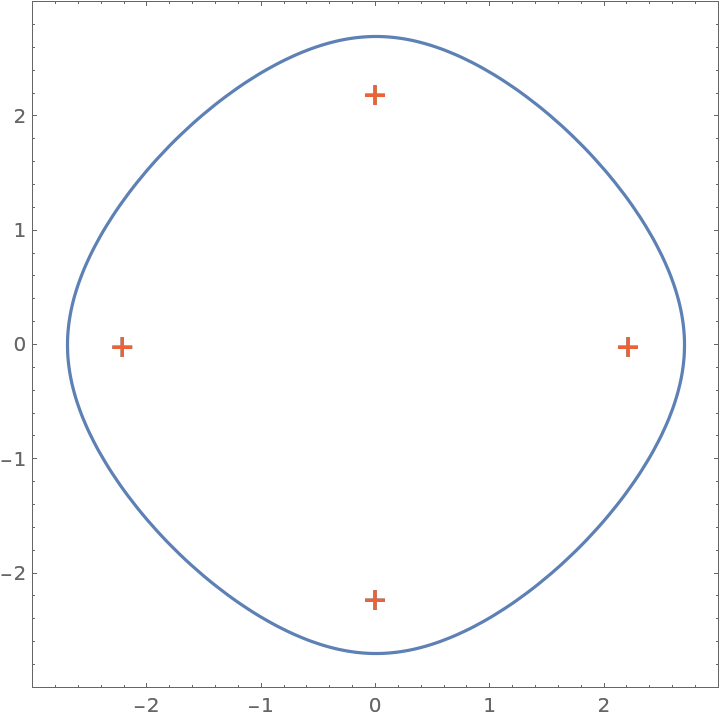 |
Evaluate MatrixFieldOfValues for a numerical matrix and a numerical value:
| In[4]:= |
| Out[4]= |
MatrixFieldOfValues works for SparseArray objects:
| In[5]:= |
| Out[5]= |
MatrixFieldOfValues threads elementwise over lists in the last argument:
| In[6]:= |
| Out[6]= |
Visualize the field of values for a large sparse matrix:
| In[7]:= | ![mat = ExampleData[{"Matrix", "DWA512"}];
ParametricPlot[
ReIm[ResourceFunction["MatrixFieldOfValues"][mat, t]], {t, 0, 2 \[Pi]}, {Axes -> None, Frame -> True, PlotRange -> All}]](https://www.wolframcloud.com/obj/resourcesystem/images/1fe/1fe15e26-4cd0-4d10-91ff-3bbf05a8b9c4/25ef2df2f40eb0bc.png) |
| Out[7]= | 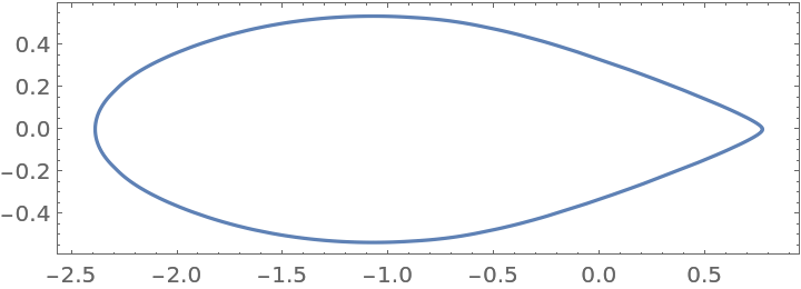 |
Brillhart's cubic:
| In[8]:= | ![ParametricPlot[ReIm[ResourceFunction["MatrixFieldOfValues"][\!\(\*
TagBox[
RowBox[{"(", "", GridBox[{
{"0", "2", "2"},
{"1", "0", "2"},
{"2", "1", "0"}
},
GridBoxAlignment->{"Columns" -> {{Center}}, "Rows" -> {{Baseline}}},
GridBoxSpacings->{"Columns" -> {
Offset[
0.27999999999999997`], {
Offset[0.7]},
Offset[0.27999999999999997`]}, "Rows" -> {
Offset[0.2], {
Offset[0.4]},
Offset[0.2]}}], "", ")"}],
Function[BoxForm`e$,
MatrixForm[BoxForm`e$]]]\), t]], {t, 0, 2 \[Pi]}, Epilog -> {AbsolutePointSize[5], Point[ReIm[Eigenvalues[N@\!\(\*
TagBox[
RowBox[{"(", "", GridBox[{
{"0", "2", "2"},
{"1", "0", "2"},
{"2", "1", "0"}
},
GridBoxAlignment->{"Columns" -> {{Center}}, "Rows" -> {{Baseline}}},
GridBoxSpacings->{"Columns" -> {
Offset[
0.27999999999999997`], {
Offset[0.7]},
Offset[0.27999999999999997`]}, "Rows" -> {
Offset[0.2], {
Offset[0.4]},
Offset[0.2]}}], "", ")"}],
Function[BoxForm`e$,
MatrixForm[BoxForm`e$]]]\)]]]}]](https://www.wolframcloud.com/obj/resourcesystem/images/1fe/1fe15e26-4cd0-4d10-91ff-3bbf05a8b9c4/005717a67593e2d9.png) |
| Out[8]= | 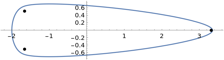 |
The field of values for a 2×2 matrix is bounded by an ellipse:
| In[9]:= |
| Out[9]= | 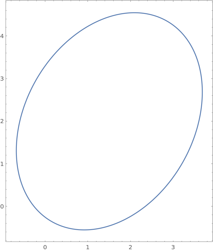 |
The field of values for a Hermitian matrix is a line segment:
| In[10]:= |
| Out[10]= | 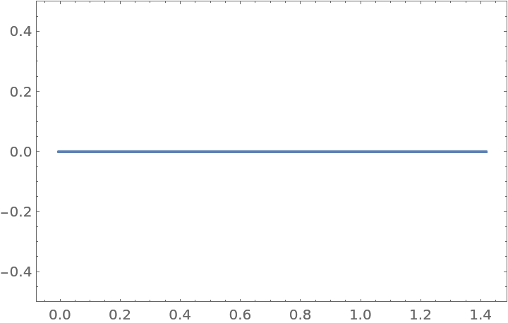 |
The field of values for a diagonal matrix is the convex hull of its eigenvalues:
| In[11]:= | ![ParametricPlot[
ReIm[ResourceFunction["MatrixFieldOfValues"][
DiagonalMatrix[{2, I, 0, -1/2, -I, -1}], t]], {t, 0, 2 \[Pi]}, {Axes -> None, Frame -> True}]](https://www.wolframcloud.com/obj/resourcesystem/images/1fe/1fe15e26-4cd0-4d10-91ff-3bbf05a8b9c4/7e55717b7ad02814.png) |
| Out[11]= | 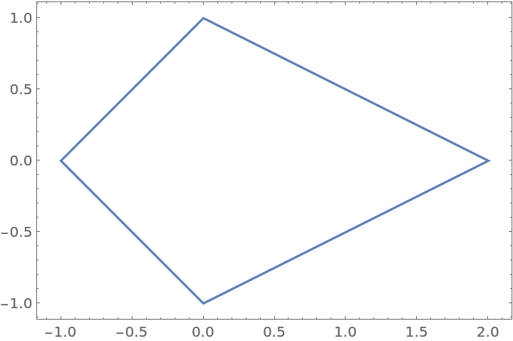 |
This work is licensed under a Creative Commons Attribution 4.0 International License