Function Repository Resource:

StereographicProjection

Source Notebook

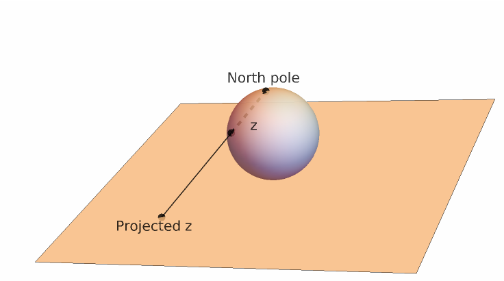
Compute the stereographic projection from the unit sphere to a plane

Contributed by: Wolfram Staff (original content by Alfred Gray)

ResourceFunction["StereographicProjection"][p]

computes the stereographic projection of the point p on the unit sphere to the plane.

Details and Options

The stereographic projection is defined as

for

∈ ℝ², where the semicolon indicates that the numerator is a vector.

The projection obtained is generated by projecting points lying on a sphere from the sphere’s north pole to a plane tangent to the south pole of the sphere and plotting the intersection of the projection segment with the plane.

The inverse of ResourceFunction["StereographicProjection"] is provided as the resource function InverseStereographicProjection.

Examples

Basic Examples (2)

An array of points:

In[1]:=

$points = Flatten[ Table[{(2 m)/(1 + m^2 + n^2), (2 n)/( 1 + m^2 + n^2), (-1 + m^2 + n^2)/(1 + m^2 + n^2)}, {m, -3, 3, .5}, {n, -3, 3, .5}], 1];$

Stereographic projection:

In[2]:=

Out[2]=

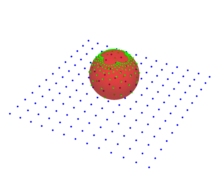
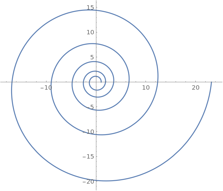
The spherical loxodrome becomes the logarithmic spiral:

In[3]:=

$loxie = ResourceFunction[ "StereographicProjection"][{(2 a E^(b t) Cos[t])/( 1 + a^2 E^(2 b t)), (2 a E^(b t) Sin[t])/( 1 + a^2 E^(2 b t)), (-1 + a^2 E^(2 b t))/(1 + a^2 E^(2 b t))}] // Simplify$

Out[3]=

Plot of the the logarithmic spiral:

In[4]:=

$ParametricPlot[loxie /. {a -> 1, b -> 1/10}, {t, 0, 10 \[Pi]}]$

Out[4]=

Applications (1)

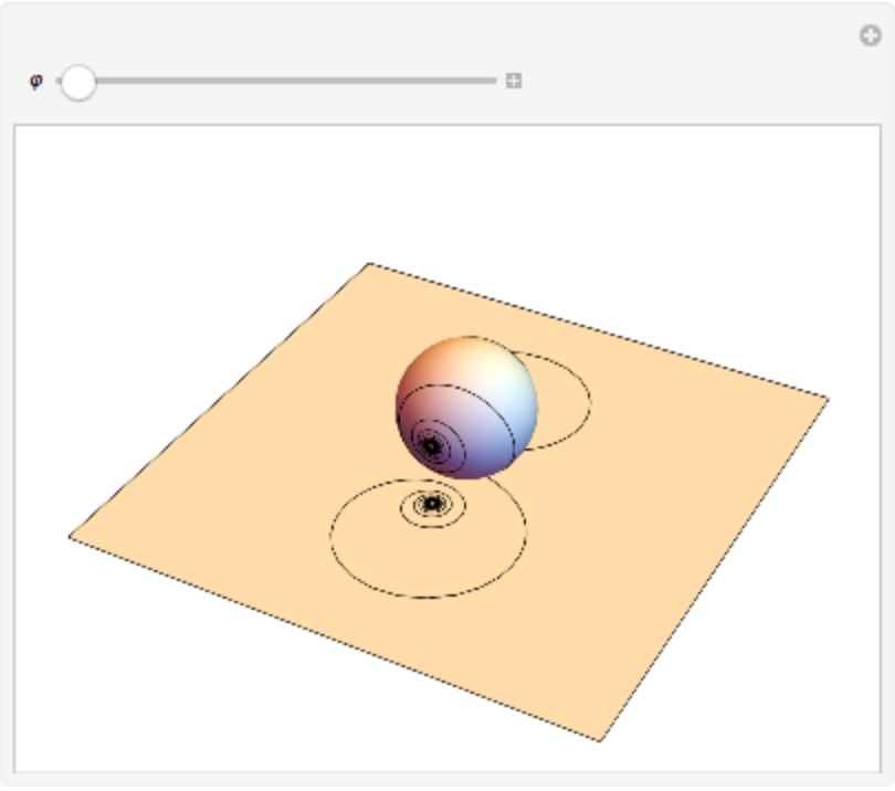
Stereographic projection of a rotated loxodrome, used for 3D printing:

In[5]:=

$Manipulate[Module[{lox, proj}, lox = ResourceFunction[ ResourceObject[ Association[{ "Name" -> "ApproximatedCurve", "ShortName" -> "ApproximatedCurve", "UUID" -> "6f76840e-ca49-453f-b718-9ebcaeb2881b", "ResourceType" -> "Function", "Version" -> "1.0.0", "Description" -> "Get an approximation to a parametric curve", "RepositoryLocation" -> URL[ "https://www.wolframcloud.com/objects/resourcesystem/api/1.\ 0"], "SymbolName" -> "FunctionRepository`$\ 549444ae0332467fb446b0981ec4a231`ApproximatedCurve", "FunctionLocation" -> CloudObject[ "https://www.wolframcloud.com/obj/1062a39e-e8ea-4b37-bc78-\ 8718bdc1c0ed"]}], {ResourceSystemBase -> Automatic}]][ RotationMatrix[\[CurlyPhi], {1, 0, 0}].{Sin[t], -t/4, -Cos[t]}/ Sqrt[1 + (t/4)^2], {t, -100, 100, 2000}, "Coordinates"]; proj = (Append[ ResourceFunction["StereographicProjection"][##1], -1] &) /@ lox; Graphics3D[{Sphere[], InfinitePlane[{{0, 0, -1}, {0, 1, -1}, {1, 0, -1}}], Line[lox], Line[proj]}, PlotRange -> {{-4, 4}, {-4, 4}, {-1, 1}}, Boxed -> False]], {\[CurlyPhi], 0., \[Pi] - \[Pi]/12, \[Pi]/12}]$

Out[5]=

Properties and Relations (1)

The inverse function:

In[6]:=

Out[6]=

Neat Examples (1)

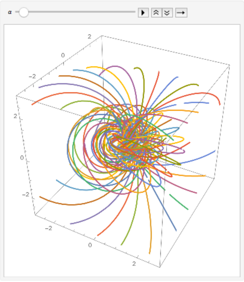
When applying a 4D to 3D stereographic projection to a Hopf fibration, a Clifford torus is generated:

In[7]:=

$HopfInverse[\[Theta]_, \[Phi]_, \[Psi]_] := {Cos[\[Phi]/ 2] Cos[\[Psi]], Cos[\[Phi]/2] Sin[\[Psi]], Cos[\[Theta] + \[Psi]] Sin[\[Phi]/2], Sin[\[Theta] + \[Psi]] Sin[\[Phi]/2]}; Ryw[\[Theta]_] := RotationMatrix[\[Theta], {{0, 0, 0, 1}, {0, 1, 0, 0}}]; Animate[ParametricPlot3D[ Evaluate[Flatten[ Table[ResourceFunction["StereographicProjection"][ Ryw[\[Alpha]].HopfInverse[\[Theta], \[Phi], \[Psi]]], {\[Phi], Pi/4, 3 Pi/4, Pi/4}, {\[Theta], 0.0, 2 Pi, Pi/9}], 1]], {\[Psi], Pi/50, 2 Pi}, PlotRange -> 3, PerformanceGoal -> "Speed"], {{\[Alpha], 0}, 0, \[Pi]}]$

Out[7]=

Publisher

Enrique Zeleny

Version History

1.0.0 – 30 June 2020

Source Metadata

Citation:
- Gray, A., Modern Differential Geometry of Curves and Surfaces with Mathematica, 2nd ed. Boca Raton, FL: CRC Press, 1997.

Related Resources

License Information

This work is licensed under a Creative Commons Attribution 4.0 International License