Wolfram Function Repository
Instant-use add-on functions for the Wolfram Language
Function Repository Resource:
Compute the parametrization of a curve projected onto the unit sphere
ResourceFunction["InverseStereographicProjection"][{u,v}] projects {u,v} from a plane onto the unit sphere. |
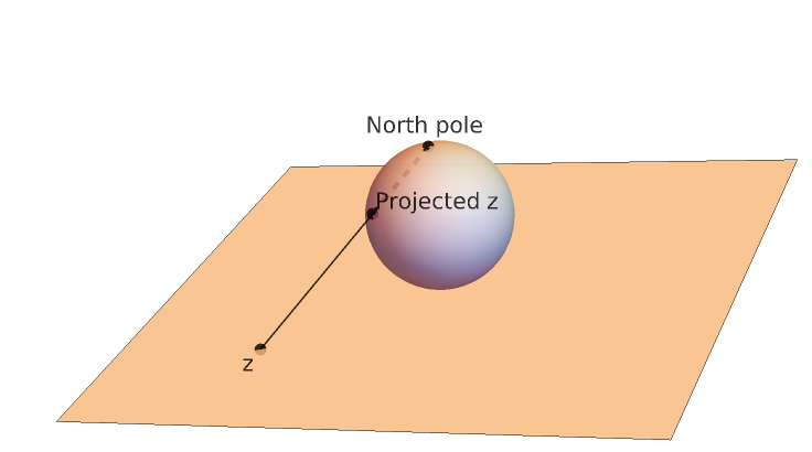
Compute the inverse stereographic projection of a generic point:
| In[1]:= |
| Out[1]= |
Define an ellipse:
| In[2]:= |
Project an ellipse onto the sphere:
| In[3]:= |
| Out[3]= |
Plot the projected ellipse:
| In[4]:= | ![Manipulate[
Show[Graphics3D[{Opacity[.5], Sphere[]}], ParametricPlot3D[
ResourceFunction["InverseStereographicProjection"][
ellipse[a, b][t]], {t, 0, 2 \[Pi]}]], {{a, 1.5}, .1, 5}, {{b, 3}, .1, 5}]](https://www.wolframcloud.com/obj/resourcesystem/images/b5a/b5ad55ea-1a32-4a5c-b73a-ddff4f22a3c3/2993a1c2b6ad7783.png) |
| Out[4]= |  |
Define a logarithmic spiral curve:
| In[5]:= |
| Out[5]= |
A plot of the logarithmic spiral:
| In[6]:= |
| Out[6]= | 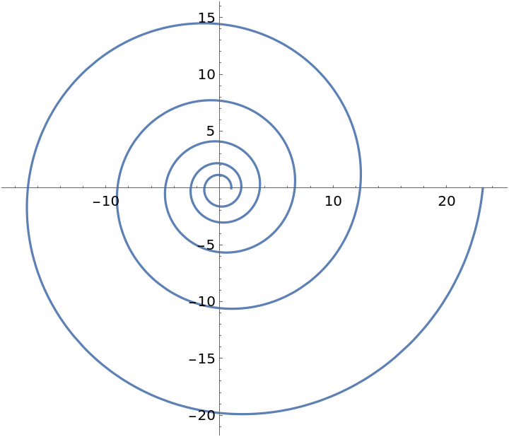 |
Project the spiral onto the sphere; it becomes a spherical loxodrome:
| In[7]:= |
| Out[7]= |
Compute the norm of the logarithmic spiral:
| In[8]:= |
| Out[8]= |
Plot the projected spiral with meridians:
| In[9]:= | ![Show[ParametricPlot3D[
Evaluate[Table[
Entity["Surface", "Sphere"]["ParametricEquations"][1][u, v], {u, 0, 2 \[Pi], \[Pi]/12}]], {v, -\[Pi], \[Pi]}, PlotStyle -> Opacity[.5], Boxed -> False, Axes -> False], ParametricPlot3D[
Evaluate[sphericalloxodrome /. {a -> 1, b -> .15}], {t, -20, 20 \[Pi]}]]](https://www.wolframcloud.com/obj/resourcesystem/images/b5a/b5ad55ea-1a32-4a5c-b73a-ddff4f22a3c3/0a9cf78b3289799b.png) |
| Out[9]= | 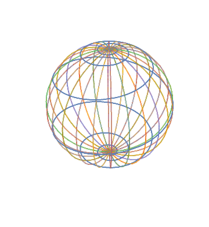 |
Plot the spherical loxodrome:
| In[10]:= | ![Manipulate[
Show[Graphics3D[{Opacity[.5], Sphere[]}], ParametricPlot3D[{(2 a E^(b t) Cos[t])/(1 + a^2 E^(2 b t)), (
2 a E^(b t) Sin[t])/(1 + a^2 E^(2 b t)), (-1 + a^2 E^(2 b t))/(
1 + a^2 E^(2 b t))}, {t, 0, 20 \[Pi]}]], {a, .1, 2}, {b, .1, 2}]](https://www.wolframcloud.com/obj/resourcesystem/images/b5a/b5ad55ea-1a32-4a5c-b73a-ddff4f22a3c3/605d1f7e876542d0.png) |
| Out[10]= | 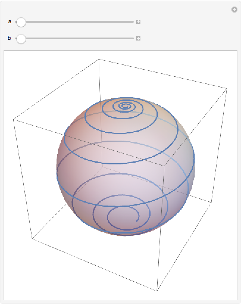 |
Define the second butterfly curve:
| In[11]:= |
| Out[11]= |
Project the curve onto the sphere:
| In[12]:= | ![proj = ResourceFunction["InverseStereographicProjection"][
Entity["PlaneCurve", "ButterflyCurve2"]["ParametricEquations"][3][
t]] // Simplify](https://www.wolframcloud.com/obj/resourcesystem/images/b5a/b5ad55ea-1a32-4a5c-b73a-ddff4f22a3c3/38b8b2d919299d69.png) |
| Out[12]= |  |
Plot the curve and the projection:
| In[13]:= | ![Show[Graphics3D[{Opacity[.5], Sphere[]}, Boxed -> False], ParametricPlot3D[proj, {t, 0, 20 \[Pi]}, PlotStyle -> Green],
ParametricPlot3D[Evaluate[Append[sbc, -1]], {t, 0, 20 \[Pi]}, PlotPoints -> 500]]](https://www.wolframcloud.com/obj/resourcesystem/images/b5a/b5ad55ea-1a32-4a5c-b73a-ddff4f22a3c3/79cdff921adbb782.png) |
| Out[13]= | 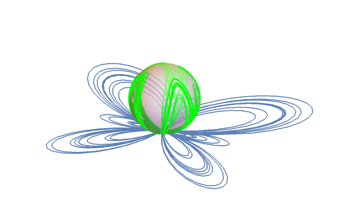 |
The norm of the stereographic sphere:
| In[14]:= |
| Out[14]= |
Project a grid of points in Cartesian coordinates:
| In[15]:= |
A Cartesian grid on the plane appears distorted on the sphere; show the points and their projections onto the sphere:
| In[16]:= | ![Show[Graphics3D[{Point[Append[#, -1] & /@ points], Green, Point[ResourceFunction["InverseStereographicProjection"] /@ points], Opacity[.5], Red, Sphere[]}, Boxed -> False]]](https://www.wolframcloud.com/obj/resourcesystem/images/b5a/b5ad55ea-1a32-4a5c-b73a-ddff4f22a3c3/435e2a6f7e6e1ac2.png) |
| Out[16]= | 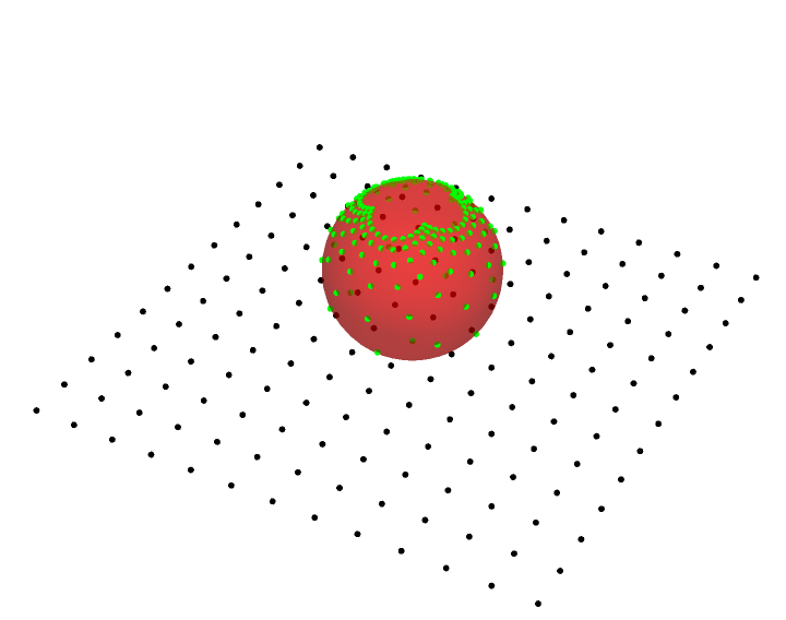 |
Project a grid of lines instead:
| In[17]:= | ![grid = Join[
Table[ResourceFunction[
"InverseStereographicProjection"][{t, n}], {n, -2, 2, .5}], Table[ResourceFunction[
"InverseStereographicProjection"][{n, t}], {n, -2, 2, .5}]];](https://www.wolframcloud.com/obj/resourcesystem/images/b5a/b5ad55ea-1a32-4a5c-b73a-ddff4f22a3c3/483fb3decba0b14b.png) |
Show the lines and their projections:
| In[18]:= | ![Show[Graphics3D[{Opacity[.5], Sphere[]}, Boxed -> False], ParametricPlot3D[Evaluate[grid], {t, -2, 2}], ParametricPlot3D[
Evaluate[Append[#, -1] & /@ Join[Table[{t, n}, {n, -2, 2, .5}], Table[{n, t}, {n, -2, 2, .5}]]], {t, -2, 2}, PlotRange -> 2]]](https://www.wolframcloud.com/obj/resourcesystem/images/b5a/b5ad55ea-1a32-4a5c-b73a-ddff4f22a3c3/5e1ffdd43770a9c5.png) |
| Out[18]= | 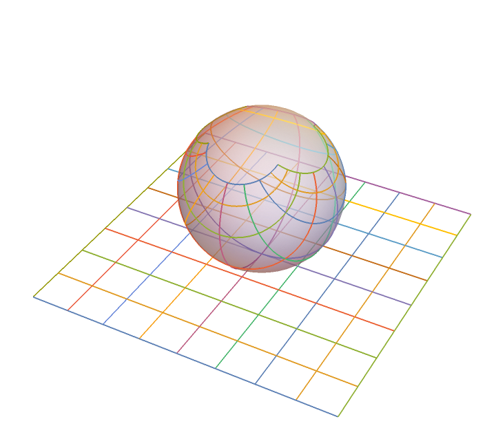 |
The same mesh can be generated by ParametricPlot3D. The grid lines are still perpendicular, but the sectors get smaller close to the north pole:
| In[19]:= | ![ParametricPlot3D[
Evaluate[ResourceFunction[
"InverseStereographicProjection"][{u, v}]], {u, -2 \[Pi], 2 \[Pi]}, {v, -2 \[Pi], 2 \[Pi]}, PlotStyle -> Opacity[.5], PlotRange -> All, PlotPoints -> 80, Boxed -> False, Axes -> False]](https://www.wolframcloud.com/obj/resourcesystem/images/b5a/b5ad55ea-1a32-4a5c-b73a-ddff4f22a3c3/31825163382fb017.png) |
| Out[19]= | 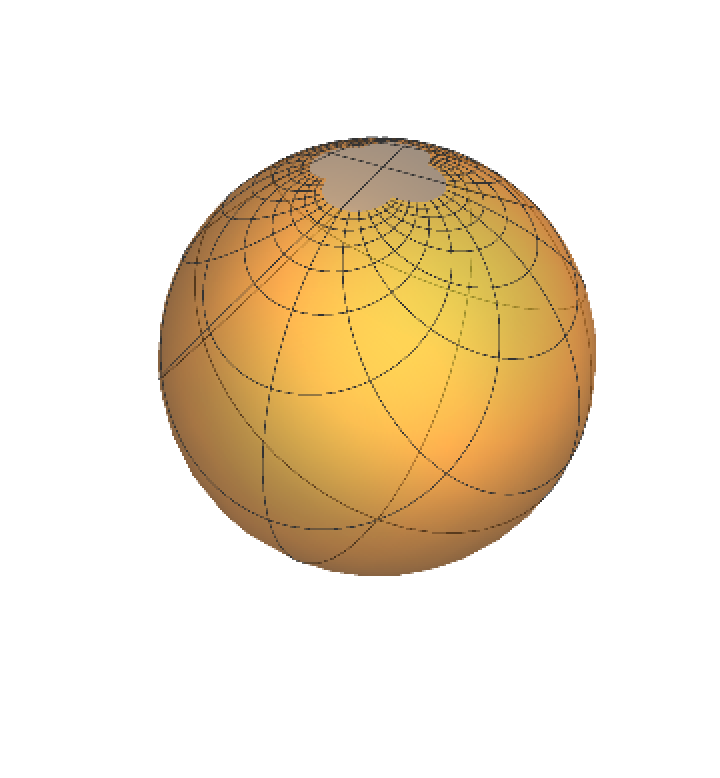 |
This work is licensed under a Creative Commons Attribution 4.0 International License