Function Repository Resource:

CountPolynomialSolutions

Source Notebook

Count the roots to a system of polynomials

Contributed by: Daniel Lichtblau

ResourceFunction["CountPolynomialSolutions"][polys,vars]

counts the number of solutions of the polynomial system given by polys in the variables vars.

ResourceFunction["CountPolynomialSolutions"][polys]

counts the number of solutions in terms of the variables in polys.

Details and Options

ResourceFunction["CountPolynomialSolutions"] counts all solutions over the complex numbers.

ResourceFunction["CountPolynomialSolutions"] counts solutions by multiplicity.

If the solution set has dimension greater than zero then ResourceFunction["CountPolynomialSolutions"] will return Infinity.

If the input has coefficients that are approximate numerical values then ResourceFunction["CountPolynomialSolutions"] will use approximate arithmetic. This can fail if precision is not sufficient for the method used.

The input for polys can be either a list of polynomials or a list of polynomial equations. In the former case the system in question is obtained by setting all polynomials to zero. The set of zeros is known as the variety defined by the polynomials.

If there are parameters then the count will be based on generic values for those parameters. For special cases the solution count might be either smaller or infinite (but never both finite and larger).

If the precision is finite and there are parameters then random values of that precision will be substituted for them before assessing the count.

If no vars are specified then the variables will be taken as Variables[polys] (so there will be no parameters in this situation). The vars list must be provided explicitly in order to have some unknowns regarded as variables.

ResourceFunction["CountPolynomialSolutions"] uses a method related to one of those used by NSolve, wherein a Gröbner basis is computed and the normal set is found.

ResourceFunction["CountPolynomialSolutions"] is typically more efficient than Solve since it does not attempt to form the solutions and also can use a (typically) more efficient term ordering.

In contrast to NSolve, ResourceFunction["CountPolynomialSolutions"] will use exact methods provided the input system is exact and WorkingPrecision is set to either Automatic (the default) or Infinity.

One can sometimes improve speed using a non-default MonomialOrder option setting.

One can count solutions in an algebraic closure of a prime field using the Modulus option. For all but finitely many primes this will agree with the solution count over the complexes. This gives a probabilistic method that is often facter than working over the complexes.

Examples

Basic Examples (3)

Count the number of solutions to a bivariate system:

In[1]:=

$polys = {x^2 - y, y^3 + y + 1}; ResourceFunction["CountPolynomialSolutions"][polys]$

Out[2]=

Compare to the number of solutions produced by Solve:

In[3]:=

Out[3]=

Compare instead to the number of solutions produced by NSolve:

In[4]:=

Out[4]=

Scope (5)

Count the solutions to a trivariate system with two polynomials of degree 3 and one of degree 4:

In[5]:=

$polys = {x^3 + 5*x*z - 2*x*y - y^2 + z^3 - 3*y^2*z, y^3 + x^2*y - 7*x*y^2 + 3*x^2 - 5*x*y - 1, x*z^2 + 4*x*y*z + y^2*z - 2*z + x^2*y*z - 11}; ResourceFunction["CountPolynomialSolutions"][polys, {x, y, z}]$

Out[6]=

Count the solutions to a larger system:

In[7]:=

$polys = {a^5 + 30*a^3*b + 40*a^2*c + 89*a*b^2 + 88*b*c, a^6 + 55*a^4*b + 80*a^3*c + 439*a^2*b^2 + 688*a*b*c + 225*b^3 + 160*c^2, a^7 + 91*a^5*b + 140*a^4*c + 1519*a^3*b^2 + 2968*a^2*b*c + 3429*a*b^3 + 1120*a*c^2 + 3708*b^2*c}; ResourceFunction["CountPolynomialSolutions"][polys, Variables[polys]]$

Out[8]=

Count the solutions to an "offset" system, wherein the polynomials are set equal to nonzero constants:

In[9]:=

Out[9]=

Coefficients need not be rational:

In[10]:=

$polys = {x0^2 + x1^2 + x2^2 - 1, x0*x3 + x1*x4 + x2*x5, x3^2 + x4^2 + x5^2 - 3/10, x3^2 + x4^2 - 2*x2*x4 + x2^2 + x5^2 + 2*x1*x5 + x1^2 - 1/4, x3^2 + Sqrt[3]*x2*x3 + 3/4*x2^2 + x4^2 - x2*x4 + 1/4*x2^2 + x5^2 - Sqrt[3]*x0*x5 + x1*x5 + 3/4*x0^2 - Sqrt[3]/2*x0*x1 + 1/4*x1^2 - 1/4, x3^2 - 2/3*Sqrt[6]*x1*x3 + Sqrt[3]/3*x2*x3 + 2/3*x1^2 - Sqrt[18]/9*x1*x2 + 1/12*x2^2 + x4^2 + 2/3*Sqrt[6]*x0*x4 - x2*x4 + 2/3*x0^2 - Sqrt[6]/3*x0*x2 + 1/4*x2^2 + x5^2 - Sqrt[3]/3*x0*x5 + x1*x5 + 1/12*x0^2 - Sqrt[3]/6*x0*x1 + 1/4*x1^2 - 1/4}; Timing[ResourceFunction["CountPolynomialSolutions"][ polys, {x0, x1, x2, x3, x4, x5}]]$

Out[11]=

This is somewhat faster than explicitly solving the system:

In[12]:=

Out[12]=

It is faster still to do the computation at modest finite precision:

In[13]:=

Out[13]=

Coefficients can be parameters, that is, unknown values:

In[14]:=

$polys = {a*x^2 - b*x*y^3, y^3 + c*x^2*y + d*x*y + e}; ResourceFunction["CountPolynomialSolutions"][polys, {x, y}]$

Out[15]=

We check that this is in fact the count for a specific set of parameter values:

In[16]:=

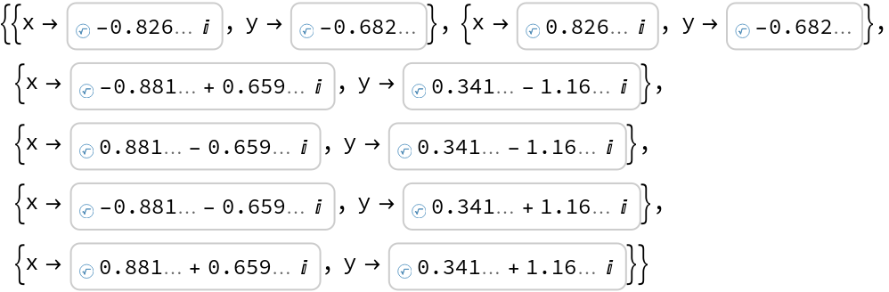
$With[{a = 12, b = -Pi^2, c = E, d = I*Pi, e = EulerGamma}, polys = {a*x^2 - b*x*y^3, y^3 + c*x^2*y + d*x*y + e}; ns = NSolve[polys, {x, y}]; {ns, Length[ns]}]$

Out[16]=

An overdetermined system often will have no solutions:

In[17]:=

$ResourceFunction[ "CountPolynomialSolutions"][{x^2 - 2*x*y + y - 3 == 0, x*y^2 == -7, x^4 + y^4 == 1}, {x, y}]$

Out[17]=

A system of n polynomials in n variables might fail to have a finite solution set:

In[18]:=

$polys = {x + x^2 + y - 2 x y - 3 x z^2, 7 + x^4 + x y^2 + y^4 + z^2, 7 - x - x^2 + 10 x^3 + 4 x^4 + x^7 - y - 19 x y + 5 x^2 y - 4 x^3 y - 3 x^5 y + 7 y^2 + 17 x y^2 - 4 x^2 y^2 + 2 x^4 y^2 + 2 x^5 y^2 - 3 x^2 y^3 + y^4 + x^2 y^4 + x^3 y^4 - y^5 - x y^5 + y^6 + 2 x y^6 - 14 y z - 2 x^4 y z - 3 x y^3 z - x^2 y^3 z - y^4 z + 2 x y^4 z - 2 y^5 z + 8 z^2 + 3 x z^2 - x^2 z^2 - 9 x^3 z^2 + x^4 z^2 - 4 x y z^2 - 4 x^2 y z^2 + y^2 z^2 + 3 x y^2 z^2 + y^4 z^2 + 3 x y^4 z^2 - 2 y z^3 + 3 x y^3 z^3 + z^4 + 3 x^2 z^4}; ResourceFunction["CountPolynomialSolutions"][polys, {x, y, z}]$

Out[19]=

If we allow z to be a parameter then the solution count is finite:

In[20]:=

Out[20]=

Options (4)

This is a test system from an ISSAC 2001 conference paper:

In[21]:=

$g0 = -84 + 41*x + 23*y + 99*x^2*y^5 - 61*x^2*y^4 - 50*x^2*y^3 - 12*x^2*y^2 - 18*x^2*y - 26*x*y^7 - 62*x*y^6 + x*y^5 - 47*x*y^4 - 91*x*y^3 - 47*x*y^2 + 66*x^3*y - 55*x^7*y - 35*x^6*y^2 + 97*x^6*y + 79*x^5*y^3 + 56*x^5*y^2 + 49*x^5*y + 57*x^4*y^4 - 59*x^4*y^3 + 45*x^4*y^2 - 8*x^4*y + 92*x^3*y^5 + 77*x^3*y^2 + 54*x^3 + 53*y^6 + 31*x^2 - 90*y^7 - 58*y^8 - 85*x^8 - 37*x^7 - 86*y^2 + 50*x^6 + 83*y^3 + 63*x^5 + 94*y^4 - 93*x^4 - y^5 - 5*x^2*y^6 - 61*x*y + 43*x^3*y^4 - 62*x^3*y^3; h0 = -76 - 53*x + 88*y + 66*x^2*y^5 - 29*x^2*y^4 - 91*x^2*y^3 - 53*x^2*y^2 - 19*x^2*y + 68*x*y^6 - 72*x*y^5 - 87*x*y^4 + 79*x*y^3 + 43*x*y^2 + 80*x^3*y - 50*x^6*y - 53*x^5*y^2 + 85*x^5*y + 78*x^4*y^3 + 17*x^4*y^2 + 72*x^4*y + 30*x^3*y^2 + 72*x^3 - 23*y^6 - 47*x^2 - 61*y^7 + 19*x^7 - 42*y^2 + 88*x^6 - 34*y^3 + 49*x^5 + 31*y^4 - 99*x^4 - 37*y^5 - 66*x*y - 85*x^3*y^4 - 86*x^3*y^3; f0 = Expand[g0*h0]; polys = {f0, D[f0, x], D[f0, y]}; vars = Variables[polys];$

It is quite slow to handle at exact precision:

In[22]:=

Out[22]=

It can be done quite efficiently at a working precision of 200 digits:

In[23]:=

Out[23]=

This is moreover several times faster than numerically solving the system at the same precision:

In[24]:=

Out[24]=

A more extreme example comes from a 2009 ISSAC conference paper:

In[25]:=

(* Evaluate this cell to get the example input *) CloudGet["https://www.wolframcloud.com/obj/5b323740-b19c-40c6-889d-d1818561b7f3"]

Out[26]=

NSolve on this example is 2-3 orders of magnitude slower:

In[27]:=

Out[27]=

Again, using a probabilistic approach, we count solutions in a certain prime field; with high probability this will agree with the total over the complexes:

In[28]:=

Out[28]=

Provide a weight matrix for the term ordering:

In[29]:=

$polys = {x^2 - y, y^3 + y + 1}; ResourceFunction["CountPolynomialSolutions"][polys, MonomialOrder -> {{1, 2}, {2, 1}}]$

Out[30]=

Use a prime modulus to count solutions for a large system:

In[31]:=

$polys = {x1^2*x3^3 + x1*x2*x3^2*x5 + x1*x2^2*x3*x4*x5*x7 + 1, x1*x2^2*x3^2*x6 + x2*x3*x4^2*x5 + x1^2 + x5 - 3, x1^3 - x5^2, x1*x2^2*x3^2 + 2, x2^2*x3*x4 + x1*x5^2 + x3^2*x7 - 5, x1^2*x4 + x2^2*x6 + 4, x1^2 + x2^2*x3 + x4^2*x5 - x7}; vars = {x1, x2, x3, x4, x5, x6, x7}; Timing[count = ResourceFunction["CountPolynomialSolutions"][polys, vars, Modulus -> Prime[1234567]]]$

Out[32]=

This can be done much faster using a monomial order that is particularly well-suited for this system:

In[33]:=

orderMat = Join[{{1, 1, 1, 1, 1, 5, 8}}, Reverse@Most[IdentityMatrix[7]]];
Timing[countb = GroebnerBasis[polys, vars, Modulus -> Prime[1234567], MonomialOrder -> orderMat];]

Out[34]=

Properties and Relations (3)

The Caprasse system has 32 distinct solutions:

In[35]:=

$polysCaprasse = {-2*x + 2*t*x*y - z + y^2*z, 2 + 4*x^2 - 10*t*y + 4*t*x^2*y - 10*y^2 + 2*t*y^3 + 4*x*z - x^3*z + 4*x*y^2*z, -x + t^2*x - 2*z + 2*t*y*z, 2 - 10*t^2 - 10*t*y + 2*t^3*y + 4*x*z + 4*t^2*x*z + 4*z^2 + 4*t*y*z^2 - x*z^3}; Length[Solve[polysCaprasse == 0]]$

Out[36]=

A count by multiplicity shows a larger value:

In[37]:=

Out[37]=

If we slightly perturb the system then Solve will find 56 distinct solutions in agreement with CountPolynomialSolutions:

In[38]:=

$perturbpolysCaprasse = {-2*x + 2*t*x*y - (100001*z)/100000 + y^2*z, 2000001/1000000 + 4*x^2 - 10*t*y + 4*t*x^2*y - 10*y^2 + 2*t*y^3 + 4*x*z - x^3*z + 4*x*y^2*z, -x + t^2*x - 2*z + 2*t*y*z, 2 - 10*t^2 - 10*t*y + 2*t^3*y + 4*x*z + 4*t^2*x*z + 4*z^2 + 4*t*y*z^2 - x*z^3}; {Length[Solve[perturbpolysCaprasse == 0]], ResourceFunction["CountPolynomialSolutions"][perturbpolysCaprasse]}$

Out[39]=

Possible Issues (4)

Inconsistent results can arise if the system (taken from this Mathematica.StackExchange post) has coefficients with low precision:

In[40]:=

$polys = {-1 + c1^2 + s1^2, -1 + c2^2 + s2^2, -1 + c3^2 + s3^2, -1 + (-0.70873 c1 + c2 - 0.70548 s1) y11, -1 + (-0.916596 c2 + c3 + 0.399814 s2) y12, -1 + (c1 + 0.808085 c3 + 0.589066 s3) y13, -1 + (c1 + 0.808085 c3 + 0.589066 s3) y21, (-0.70548 c1 + 0.70873 s1 + s2) y11 - (-0.589066 c3 + s1 + 0.808085 s3) y21, -1 + (-0.70873 c1 + c2 - 0.70548 s1) y22, (0.399814 c2 + 0.916596 s2 + s3) y12 - (-0.70548 c1 + 0.70873 s1 + s2) y22, -1 + (-0.916596 c2 + c3 + 0.399814 s2) y23, (0.589066 c3 - s1 - 0.808085 s3) y13 - (0.399814 c2 + 0.916596 s2 + s3) y23}; ResourceFunction["CountPolynomialSolutions"][polys, Variables[polys]]$

Out[41]=

We can get a different count by raising the precision:

In[42]:=

Out[42]=

As is indicated in the StackExchange thread, there are further subtleties-- six of the eight solutions are quite large:

In[43]:=

Out[44]=

This is because the exact system from which this was taken lives on the "discriminant variety" for systems with the same polynomial structure but having generic coefficients. Had we an exact form for the coefficients, these six would not be present (they go to infinity as the coefficients approach the discriminant variety).

One can isolate to the two expected solutions with some amount of trial and error in setting the Tolerance option of GroebnerBasis:

In[45]:=

SetOptions[GroebnerBasis, Tolerance -> 10^(-4)];
ResourceFunction["CountPolynomialSolutions"][
SetPrecision[polys, 200]]
SetOptions[GroebnerBasis, Tolerance -> 0];

Out[46]=

Requirements

Wolfram Language 13.0 (December 2021) or above

Version History

1.1.0 – 03 May 2024
1.0.1 – 07 August 2023
1.0.0 – 08 May 2023

Source Metadata

Citation:
- R. Corless. Editor’s corner: Groebner bases and matrix eigenproblems.
  Sigsam Bulletin: Communications in Computer Algebra 30(4), December 1996, 26-32.
- D. Lichtblau. Solving polynomial systems using numeric Gröbner bases. 6th International Conference, South Bend, IN, USA, July 24-27, 2018, Proceedings. In: Davenport, J., Kauers, M., Labahn, G., Urban, J. (eds) Mathematical Software – ICMS 2018. ICMS 2018. Lecture Notes in Computer Science(), vol 10931. Springer, Cham. DOI: 10.1007/978-3-319-96418-8_40

Related Resources

License Information

This work is licensed under a Creative Commons Attribution 4.0 International License

Wolfram Function Repository

CountPolynomialSolutions

Details and Options