Wolfram Language
Paclet Repository
Community-contributed installable additions to the Wolfram Language
Primary Navigation
Categories
Cloud & Deployment
Core Language & Structure
Data Manipulation & Analysis
Engineering Data & Computation
External Interfaces & Connections
Financial Data & Computation
Geographic Data & Computation
Geometry
Graphs & Networks
Higher Mathematical Computation
Images
Knowledge Representation & Natural Language
Machine Learning
Notebook Documents & Presentation
Scientific and Medical Data & Computation
Social, Cultural & Linguistic Data
Strings & Text
Symbolic & Numeric Computation
System Operation & Setup
Time-Related Computation
User Interface Construction
Visualization & Graphics
Random Paclet
Alphabetical List
Using Paclets
Create a Paclet
Get Started
Download Definition Notebook
Learn More about
Wolfram Language
RobustBackSteppingCancellation
Guides
Guide to ZigangPan`RobustBackSteppingCancellation`
Symbols
linearFactorConvex
RobustBackSteppingArztanG
RobustBackSteppingArztan
RobustBackSteppingCancellationG
RobustBackSteppingCancellation
ZigangPan`RobustBackSteppingCancellation`
R
o
b
u
s
t
B
a
c
k
S
t
e
p
p
i
n
g
C
a
n
c
e
l
l
a
t
i
o
n
G
{
V
,
α
,
x
,
σ
}
=
R
o
b
u
s
t
B
a
c
k
S
t
e
p
p
i
n
g
C
a
n
c
e
l
l
a
t
i
o
n
G
[
V
o
,
α
o
,
f
o
,
h
o
,
f
a
,
g
a
,
h
a
,
x
o
,
x
a
,
x
d
,
Γ
,
Φ
f
u
n
,
Δ
f
u
n
]
T
h
i
s
i
s
a
n
i
m
p
l
e
m
e
n
t
a
t
i
o
n
o
f
t
h
e
b
a
c
k
s
t
e
p
p
i
n
g
L
e
m
m
a
w
i
t
h
d
i
r
e
c
t
c
a
n
c
e
l
l
a
t
i
o
n
a
n
d
w
i
t
h
a
m
o
r
e
g
e
n
e
r
a
l
c
o
s
t
s
t
r
u
c
t
u
r
e
o
n
t
h
e
d
i
s
t
u
r
b
a
n
c
e
i
n
p
u
t
s
a
n
d
t
h
e
a
s
s
u
m
p
t
i
o
n
t
h
a
t
f
o
[
x
o
,
x
a
,
x
d
]
a
n
d
h
o
[
x
o
,
x
a
,
x
d
]
a
r
e
l
i
n
e
a
r
i
n
x
a
.
N
o
t
a
t
i
o
n
:
x
o
:
s
t
a
t
e
v
e
c
t
o
r
f
o
r
p
r
e
v
i
o
u
s
s
u
b
s
y
s
t
e
m
(
v
e
c
t
o
r
)
x
a
:
t
h
e
a
t
t
a
t
c
h
e
d
s
t
a
t
e
(
v
i
r
t
u
a
l
c
o
n
t
r
o
l
)
(
v
e
c
t
o
r
)
x
d
:
a
d
d
i
t
i
o
n
a
l
v
a
r
i
a
b
l
e
s
i
n
d
y
n
a
m
i
c
s
(
v
e
c
t
o
r
)
S
y
s
t
e
m
:
d
x
o
/
d
t
=
f
o
[
x
o
,
x
a
,
x
d
]
+
h
o
[
x
o
,
x
a
,
x
d
]
w
d
x
a
/
d
t
=
f
a
[
x
o
,
x
a
,
x
d
]
+
g
a
[
x
o
,
x
a
,
x
d
]
u
+
h
a
[
x
o
,
x
a
,
x
d
]
w
f
o
i
s
a
v
e
c
t
o
r
,
h
o
i
s
a
m
a
t
r
i
x
,
f
a
i
s
a
v
e
c
t
o
r
,
g
a
i
s
a
s
q
u
a
r
e
m
a
t
r
i
x
,
h
a
i
s
a
m
a
t
r
i
x
.
W
e
a
s
s
u
m
e
t
h
a
t
a
v
a
l
u
e
f
u
n
c
t
i
o
n
V
o
[
x
o
]
(
s
c
a
l
a
r
)
a
n
d
a
c
o
n
t
r
o
l
l
a
w
x
a
=
α
o
[
x
o
]
(
v
e
c
t
o
r
)
h
a
v
e
b
e
e
n
c
o
m
p
u
t
e
d
f
o
r
t
h
e
x
o
d
y
n
a
m
i
c
s
t
h
a
t
a
c
h
i
e
v
e
s
t
∫
0
(
l
o
[
x
o
[
τ
]
,
x
d
[
τ
]
]
-
w
[
τ
]
.
Γ
[
x
o
[
τ
]
]
.
w
[
τ
]
)
τ
≤
V
o
[
x
0
[
0
]
]
;
∀
t
≥
0
a
n
d
f
o
r
a
n
y
w
a
v
e
f
o
r
m
o
f
w
.
T
h
i
s
b
a
c
k
s
t
e
p
p
i
n
g
c
o
m
m
a
n
d
c
o
m
p
u
t
e
s
a
v
a
l
u
e
f
u
n
c
t
i
o
n
V
,
a
c
o
n
t
r
o
l
l
a
w
α
f
o
r
u
,
t
h
e
s
t
a
t
e
v
e
c
t
o
r
i
s
x
=
F
l
a
t
t
e
n
[
{
x
o
,
x
a
,
x
d
}
]
,
a
n
d
t
h
e
c
o
r
r
e
s
p
o
n
d
i
n
g
w
o
r
s
t
c
a
s
e
d
i
s
t
u
r
b
a
n
c
e
l
a
w
σ
f
o
r
w
.
V
o
:
i
s
a
v
a
l
u
e
f
u
n
c
t
i
o
n
d
e
s
i
g
n
e
d
f
o
r
x
o
s
y
s
t
e
m
.
α
o
:
t
h
e
v
i
r
t
u
a
l
c
o
n
t
r
o
l
l
a
w
f
o
r
x
a
Γ
:
d
e
s
i
r
e
d
d
i
s
t
u
r
b
a
n
c
e
a
t
t
e
n
u
a
t
i
o
n
l
e
v
e
l
(
a
m
a
t
r
i
x
)
Φ
f
u
n
:
T
h
e
a
d
d
i
t
i
o
n
a
l
n
e
g
a
t
i
v
e
d
r
i
f
t
i
n
t
h
e
d
e
s
i
g
n
.
Δ
f
u
n
:
T
h
e
a
d
d
i
t
i
o
n
a
l
q
u
a
d
r
a
t
i
c
k
e
r
n
e
l
i
n
t
h
e
v
a
l
u
e
f
u
n
c
t
i
o
n
V
:
V
=
V
o
+
(
x
a
-
α
o
[
x
o
]
)
'
Δ
f
u
n
(
x
a
-
α
o
[
x
o
]
)
T
h
e
n
,
t
h
e
d
e
s
i
g
n
a
c
h
i
e
v
e
s
t
∫
0
(
l
o
[
x
o
[
τ
]
,
x
d
[
τ
]
]
+
(
x
a
[
τ
]
-
α
o
[
x
o
[
τ
]
]
)
'
Φ
f
u
n
[
x
o
[
τ
]
,
x
a
[
τ
]
,
x
d
[
τ
]
]
-
w
[
τ
]
.
Γ
[
x
o
[
τ
]
]
.
w
[
τ
]
)
τ
≤
V
[
x
o
〚
0
〛
,
x
a
〚
0
〛
]
∀
t
≥
0
a
n
d
f
o
r
a
n
y
w
a
v
e
o
r
m
o
f
w
.
V
,
α
,
σ
,
V
o
,
α
o
,
f
o
,
h
o
,
f
a
,
g
a
,
h
a
,
Γ
,
Φ
f
u
n
,
Δ
f
u
n
a
r
e
f
o
r
m
u
l
a
s
r
a
t
h
e
r
t
h
a
n
f
u
n
c
t
i
o
n
s
.
Examples
(
1
)
Basic Examples
(
1
)
I
n
[
1
]
:
=
N
e
e
d
s
[
"
Z
i
g
a
n
g
P
a
n
`
E
x
a
m
p
l
e
s
`
"
]
I
n
[
2
]
:
=
N
e
e
d
s
[
"
Z
i
g
a
n
g
P
a
n
`
D
i
f
f
e
r
e
n
t
i
a
l
E
q
u
a
t
i
o
n
S
o
l
v
e
r
`
"
]
I
n
[
3
]
:
=
x
c
=
{
x
1
,
x
2
,
x
3
,
x
4
}
;
$
A
s
s
u
m
p
t
i
o
n
s
=
a
s
s
u
m
e
R
e
a
l
[
x
c
]
O
u
t
[
3
]
=
x
1
∈
&
&
x
2
∈
&
&
x
3
∈
&
&
x
4
∈
I
n
[
4
]
:
=
f
e
[
x
1
_
,
x
2
_
,
x
3
_
,
x
4
_
]
:
=
{
x
3
+
x
1
^
2
,
x
1
*
x
2
+
x
4
,
x
1
*
x
3
,
x
2
*
x
4
}
I
n
[
5
]
:
=
g
e
[
x
1
_
,
x
2
_
,
x
3
_
,
x
4
_
]
:
=
{
{
0
,
0
}
,
{
0
,
0
}
,
{
1
,
0
}
,
{
0
,
-
1
}
}
I
n
[
6
]
:
=
h
e
[
x
1
_
,
x
2
_
,
x
3
_
,
x
4
_
]
:
=
{
{
1
,
0
}
,
{
-
1
,
x
1
}
,
{
0
,
0
}
,
{
1
,
1
}
}
I
n
[
7
]
:
=
V
0
=
0
;
α
0
=
{
0
,
0
}
;
γ
=
4
;
f
=
A
p
p
l
y
[
f
e
,
x
c
]
;
g
=
A
p
p
l
y
[
g
e
,
x
c
]
;
h
=
A
p
p
l
y
[
h
e
,
x
c
]
;
I
n
[
8
]
:
=
{
V
1
,
α
1
,
x
,
σ
}
=
R
o
b
u
s
t
B
a
c
k
S
t
e
p
p
i
n
g
C
a
n
c
e
l
l
a
t
i
o
n
G
[
V
0
,
α
0
,
{
}
,
{
}
,
f
〚
1
;
;
2
〛
/
.
{
x
3
0
,
x
4
0
}
,
D
[
f
〚
1
;
;
2
〛
,
{
{
x
3
,
x
4
}
}
]
,
h
〚
1
;
;
2
,
A
l
l
〛
,
{
}
,
{
x
1
,
x
2
}
,
{
}
,
γ
^
2
*
{
{
1
,
1
/
2
}
,
{
1
/
2
,
2
}
}
,
{
x
1
,
x
2
}
,
I
d
e
n
t
i
t
y
M
a
t
r
i
x
[
2
]
/
2
]
O
u
t
[
8
]
=
2
x
1
2
+
2
x
2
2
,
-
x
1
-
2
x
1
+
1
4
-
x
1
1
4
-
-
1
1
4
-
x
1
5
6
x
2
,
-
x
2
-
x
1
x
2
+
1
4
-
-
1
1
4
-
x
1
5
6
x
1
-
1
1
4
+
x
1
5
6
+
1
5
6
+
x
1
2
8
x
1
x
2
,
{
x
1
,
x
2
}
,
1
2
x
1
1
4
+
-
1
1
4
-
x
1
5
6
x
2
,
1
2
-
x
1
5
6
+
1
5
6
+
x
1
2
8
x
2
I
n
[
9
]
:
=
{
V
,
α
,
x
,
σ
}
=
R
o
b
u
s
t
B
a
c
k
S
t
e
p
p
i
n
g
C
a
n
c
e
l
l
a
t
i
o
n
G
[
V
1
,
α
1
,
f
〚
1
;
;
2
〛
,
h
〚
1
;
;
2
,
A
l
l
〛
,
f
〚
3
;
;
4
〛
,
g
〚
3
;
;
4
,
A
l
l
〛
,
h
〚
3
;
;
4
,
A
l
l
〛
,
{
x
1
,
x
2
}
,
{
x
3
,
x
4
}
,
{
}
,
γ
^
2
*
{
{
1
,
1
/
2
}
,
{
1
/
2
,
2
}
}
,
{
x
1
,
x
2
}
-
α
1
,
1
/
2
*
I
d
e
n
t
i
t
y
M
a
t
r
i
x
[
2
]
]
;
I
n
[
1
0
]
:
=
c
l
o
s
e
d
l
o
o
p
d
y
n
a
m
i
c
s
=
F
o
r
m
u
l
a
T
o
F
u
n
c
t
i
o
n
[
x
c
,
f
+
g
.
α
+
h
.
{
0
,
0
}
]
;
I
n
[
1
1
]
:
=
s
o
l
=
R
u
n
g
e
K
u
t
t
a
4
5
[
c
l
o
s
e
d
l
o
o
p
d
y
n
a
m
i
c
s
,
0
,
{
-
2
,
2
.
,
1
,
0
}
,
2
0
,
1
/
1
0
]
;
1
0
%
c
o
m
p
l
e
t
e
d
.
2
0
%
c
o
m
p
l
e
t
e
d
.
3
0
%
c
o
m
p
l
e
t
e
d
.
4
0
%
c
o
m
p
l
e
t
e
d
.
5
0
%
c
o
m
p
l
e
t
e
d
.
6
0
%
c
o
m
p
l
e
t
e
d
.
7
0
%
c
o
m
p
l
e
t
e
d
.
8
0
%
c
o
m
p
l
e
t
e
d
.
9
0
%
c
o
m
p
l
e
t
e
d
.
1
0
0
%
c
o
m
p
l
e
t
e
d
.
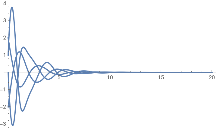
I
n
[
1
2
]
:
=
P
l
o
t
[
s
o
l
[
t
]
,
{
t
,
0
,
2
0
}
,
P
l
o
t
R
a
n
g
e
A
l
l
]
O
u
t
[
1
2
]
=
I
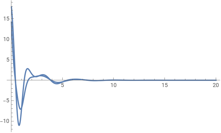
n
[
1
3
]
:
=
P
l
o
t
[
A
p
p
l
y
[
F
o
r
m
u
l
a
T
o
F
u
n
c
t
i
o
n
[
x
c
,
α
]
,
s
o
l
[
t
]
]
,
{
t
,
0
,
2
0
}
,
P
l
o
t
R
a
n
g
e
A
l
l
]
O
u
t
[
1
3
]
=
S
e
e
A
l
s
o
R
o
b
u
s
t
B
a
c
k
S
t
e
p
p
i
n
g
C
a
n
c
e
l
l
a
t
i
o
n
▪
R
o
b
u
s
t
B
a
c
k
S
t
e
p
p
i
n
g
A
r
z
t
a
n
▪
R
o
b
u
s
t
B
a
c
k
S
t
e
p
p
i
n
g
A
r
z
t
a
n
G
"
"