Wolfram Language Paclet Repository

Community-contributed installable additions to the Wolfram Language
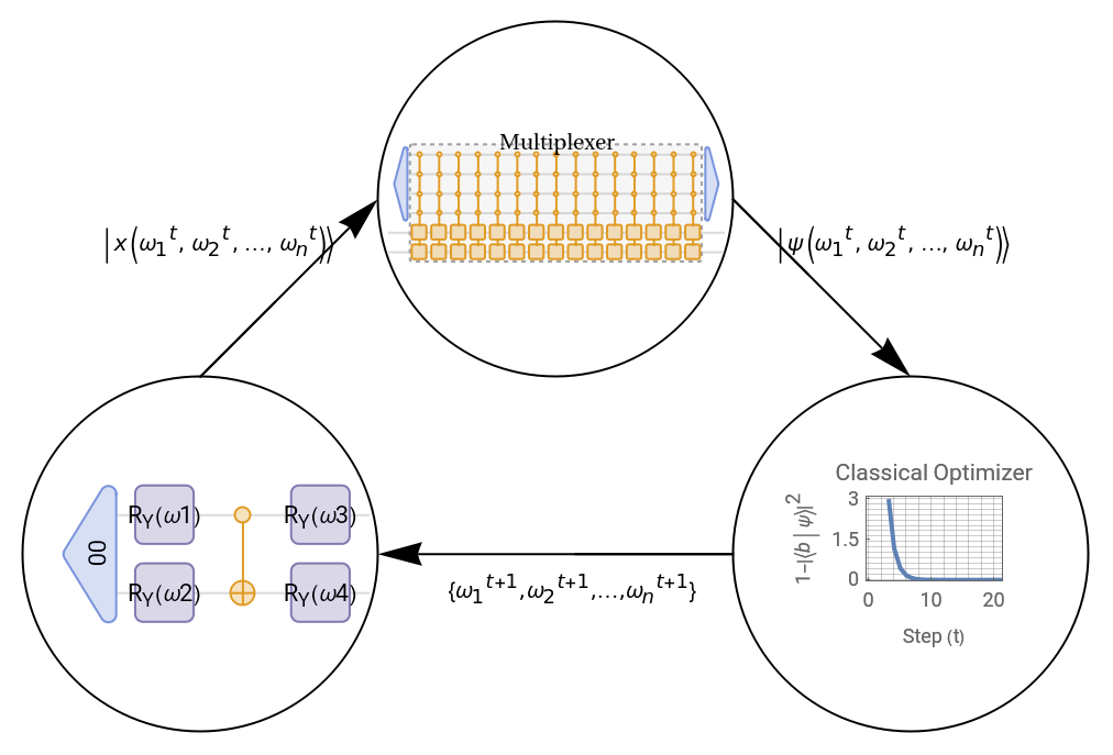
Primary Navigation

    • Cloud & Deployment
    • Core Language & Structure
    • Data Manipulation & Analysis
    • Engineering Data & Computation
    • External Interfaces & Connections
    • Financial Data & Computation
    • Geographic Data & Computation
    • Geometry
    • Graphs & Networks
    • Higher Mathematical Computation
    • Images
    • Knowledge Representation & Natural Language
    • Machine Learning
    • Notebook Documents & Presentation
    • Scientific and Medical Data & Computation
    • Social, Cultural & Linguistic Data
    • Strings & Text
    • Symbolic & Numeric Computation
    • System Operation & Setup
    • Time-Related Computation
    • User Interface Construction
    • Visualization & Graphics
    • Random Paclet
    • Alphabetical List
  • Using Paclets
    • Get Started
    • Download Definition Notebook
  • Learn More about Wolfram Language

QuantumFramework

Tutorials

  • Getting Started

Guides

  • Wolfram Quantum Computation Framework

Tech Notes

  • Bell's Theorem
  • Circuit Diagram
  • Quantum Optimization
  • Exploring Fundamentals of Quantum Theory
  • Quantum object abstraction
  • Second Quantization Functions
  • Tensor Network
  • Quantum Computation

Symbols

  • QuantumBasis
  • QuantumChannel
  • QuantumCircuitMultiwayGraph [EXPERIMENTAL]
  • QuantumCircuitOperator
  • QuantumDistance
  • QuantumEntangledQ
  • QuantumEntanglementMonotone
  • QuantumEvolve
  • QuantumMeasurement
  • QuantumMeasurementOperator
  • QuantumMeasurementSimulation
  • QuantumMPS [EXPERIMENTAL]
  • QuantumOperator
  • QuantumPartialTrace
  • QuantumPhaseSpaceTransform
  • QuantumShortcut [EXPERIMENTAL]
  • QuantumStateEstimate [EXPERIMENTAL]
  • QuantumState
  • QuantumTensorProduct
  • QuantumWignerMICTransform [EXPERIMENTAL]
  • QuantumWignerTransform [EXPERIMENTAL]
  • QuditBasis
  • QuditName
Quantum Optimization
Gradient-Based Optimization Methods
Examples Custom Functions
Quantum Linear Solver
​
In this Tech Note, we document the implementation and utilization of essential functions used in the
Wolfram Language Example Repository
for Quantum Optimization algorithms.
By providing a comprehensive overview and usage guidelines for these functions, we aim to introduce new and experienced users into quantum optimization techniques and quantum computing research.
In[92]:=
<<Wolfram`QuantumFramework`ExampleRepository`
Gradient-Based Optimization Methods
Quantum Linear Solver
The Variational Quantum Linear Solver (VQLS) is a hybrid quantum-classical technique designed to address Quantum Linear Systems Problems (QLSP). The main goal is to find linear solutions for systems as
m.x=b
.
In this Tech Note we will explain the applications and options of
QuantumLinearSolve
function implemented in the Wolfram Quantum Computation Framework to solve QLSP problems.
QuantumLinearSolve
[m,b,opts]
uses a hybrid optimization algorithm to find a quantum state described by the state vector
x
that satisfies
m.x=b
.
QuantumLinearSolve
[m,b,prop,opts]
solves
m.x=b
by including the specified properties
prop
.
We will briefly demonstrate how to apply all these functions in Wolfram quantum framework.

Details and Options

QuantumLinearSolve works on numerical matrices. The argument b must be a vector, while the argument m must be a square matrix. QuantumLinearSolve is able to compute solutions for
n
2
–dimension problems.
QuantumLinearSolve utilizes a multiplexer-based variational quantum linear solver algorithm. The primary distinctions from a conventional variational quantum linear solver algorithm are as follows:
◼
  • The multiplication of the matrix
    m
    is implemented by a multiplexer, enabling the accurate representation of the operation
    A.x
    within the quantum circuit.
  • ◼
  • The solution to the linear system is encoded directly in the amplitudes of the resultant quantum state.
  • This approach simplifies the standard variational quantum linear solver by reducing the need for multiple circuits used in the real-imaginary decomposition of the solution and the term-by-term computation within quantum circuits. A detailed step-by-step implementation is outlined in this documentation.
    The basic steps to implement the algorithm are the following:
    ◼
  • Start with a variational circuit ansatz
    V(
    ω
    i
    )
    or directly an state ansatz
    x(
    ω
    i
    )=V(
    ω
    i
    )|0〉
  • ◼
  • Apply the multiplexer to perform
    m.x(
    ω
    i
    )
    and obtain resultant
    ψ(
    ω
    i
    )
    state
  • ◼
  • Use
    ψ(
    ω
    i
    )
    state as the input for the optimizer with the cost function
    f(ω)=1-
    b
    
    ψ(ω)
    
    2
    to obtain new
    ω
    j
    parameters
  • ◼
  • Use new
    ω
    j
    parameters with the variational circuit
    V(
    ω
    i
    )
    or state ansatz
    x(
    ω
    j
    )
  • ◼
  • Repeat the process until you obtain
    f(
    ω
    opt
    )=1-
    b
    
    ψ(
    ω
    opt
    )
    
    2
    =0
  • Algorithm Implementation

    Ansatz
    Multiplexer
    Cost Function

    Options

    "Ansatz"
    Automatic
    use specified ansatz instead of the one generated by the function
    "GlobalPhaseAccuracy"
    -5
    10
    expected accuracy for global phase estimation
    AccuracyGoal
    Automatic
    number of digits of final accuracy sought
    MaxIterations
    Automatic
    maximum number of iterations to use
    Method
    Automatic
    method to use
    PrecisionGoal
    Automatic
    number of digits of final precision sought
    WorkingPrecision
    MachinePrecision
    the precision used in internal computations
    Ansatz
    GlobalPhaseAccuracy
    AccuracyGoal & PrecisionGoal
    Method
    Heuristic methods include:
    "NelderMead"
    use only convex methods
    "DifferentialEvolution"
    use differential evolution
    "SimulatedAnnealing"
    use simulated annealing
    "RandomSearch"
    use the best local minimum found from multiple random starting points
    "Couenne"
    use the Couenne library for non-convex mixed-integer nonlinear problems
    Plot progression is shown when using methods other than
    Automatic
    :
    In[10]:=
    m=RandomReal[{0,1},{4,4}]
    Out[10]=
    {{0.00393484,0.726178,0.647708,0.486648},{0.425836,0.192925,0.135447,0.156309},{0.0473378,0.134998,0.214507,0.380623},{0.916129,0.637982,0.761709,0.375096}}
    In[11]:=
    b=RandomReal[{0,1},4]
    Out[11]=
    {0.383922,0.335146,0.175575,0.653389}
    In[12]:=
    QuantumLinearSolve[m,b,Method"DifferentialEvolution"]
    Out[12]=
    {0.477453+0.,0.67417+0.,-0.500057+0.,0.444606+0.}
    Some methods may give suboptimal results for certain problems:
    In[13]:=
    solutions=(#QuantumLinearSolve[m,b,Method#])&/@{Automatic,"NelderMead","DifferentialEvolution","SimulatedAnnealing"};
    QuantumLinearSolve
    ::error
    :Global phase deviation exceeds threshold; possible errors.
    ​
    In[14]:=
    solutions//TableForm
    Out[14]//TableForm=
    Automatic{0.477453+0.,0.67417+0.,-0.500057+0.,0.444606+0.}
    NelderMead{0.477453+0.,0.674175+0.,-0.500064+0.,0.444607+0.}
    DifferentialEvolution{0.477453+0.,0.67417+0.,-0.500057+0.,0.444606+0.}
    SimulatedAnnealing{0.477453+0.,0.674171+0.,-0.500058+0.,0.444607+0.}
    WorkingPrecision

    Example

    Simple example
    Generate a random 4×4 real matrix:
    In[93]:=
    m=RandomReal[{0,1},{4,4}];​​m//MatrixForm
    Out[94]//MatrixForm=
    0.596166
    0.62566
    0.816575
    0.857365
    0.287865
    0.236078
    0.491353
    0.593494
    0.786389
    0.0297055
    0.638947
    0.00472644
    0.736549
    0.108758
    0.314166
    0.0812839
    Generate a random complex vector of the length 4:
    In[95]:=
    b=RandomComplex[{-0.1-0.1I,0.1+0.1I},4]
    Out[95]=
    {0.0170825+0.049994,0.027093+0.091541,0.0806183-0.0000258573,-0.0829871-0.0489408}
    Use them as input in the
    QuantumLinearSolve
    :
    In[99]:=
    QuantumLinearSolve[m,b]
    Out[99]=
    {-0.287755-0.110093,-0.0772302-0.274276,0.485296+0.146765,-0.185835+0.195234}
    When running above code, you may see a progress box describing steps and estimated time.
    Compare the results:
    Properties
    You can request the components used during the calculation using a third property argument:
    Show the ansatz quantum state used for parameter optimization"
    Show the quantum circuit used for parameter optimization:
    Request more than one property:
    Examples Custom Functions

    © 2025 Wolfram. All rights reserved.

    • Legal & Privacy Policy
    • Contact Us
    • WolframAlpha.com
    • WolframCloud.com