Wolfram Function Repository
Instant-use add-on functions for the Wolfram Language
Function Repository Resource:
Compute the control points of a Bézier curve that interpolates a given set of points
ResourceFunction["BezierInterpolatingControlPoints"][{x1,x2,…},{f1,f2,…}] gives the Bernstein basis coefficients of the interpolating polynomial for the function values fi corresponding to x values xi. | |
ResourceFunction["BezierInterpolatingControlPoints"][{t1,t2,…},{{x1,y1,…},{x2,y2,…},…}] generates the control points for a full-degree interpolating Bézier curve with interpolation nodes ti and points {xi,yi,…}. |
A list of points:
| In[1]:= |
Get the coefficients of the Bézier interpolant:
| In[2]:= |
| Out[2]= |
Plot the Bézier interpolant along with the points:
| In[3]:= |
| Out[3]= | 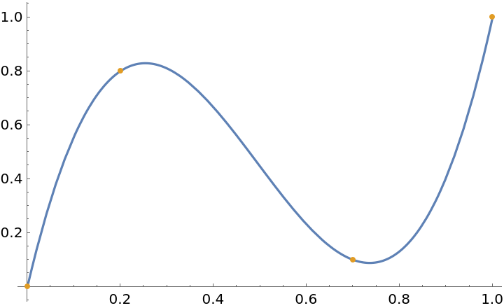 |
A set of points to interpolate:
| In[4]:= |
Generate the Bézier control points:
| In[5]:= |
| Out[5]= |
Show the Bézier curve along with the points:
| In[6]:= | ![Graphics[{{Directive[AbsoluteThickness[2], ColorData[97, 1]], BezierCurve[cp, SplineDegree -> (Length[pts] - 1)]}, {Directive[
AbsolutePointSize[6], ColorData[97, 4]], Point[pts]}}, Sequence[
PlotRange -> {{0., 5.}, {0., 3.}}, PlotRangePadding -> Scaled[0.1]]]](https://www.wolframcloud.com/obj/resourcesystem/images/ffd/ffd1599e-8282-4793-b7ab-741577254934/73e6d5a9f2decfc1.png) |
| Out[6]= | 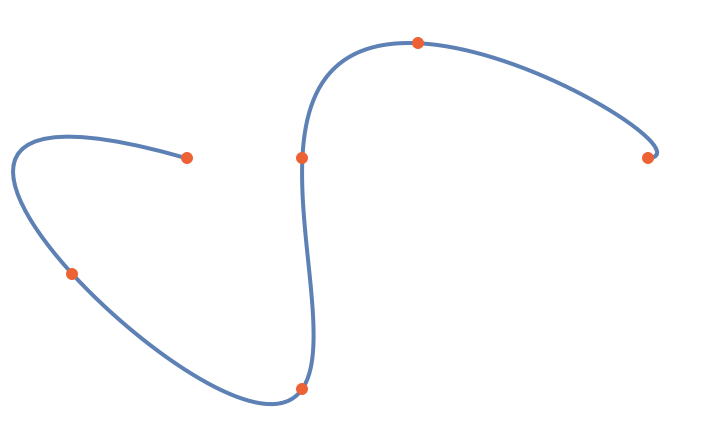 |
Use BezierInterpolatingControlPoints to generate an interpolating Bézier surface patch:
| In[7]:= | ![xl = {0., 1./3, 0.8, 1.}; yl = {0., 0.2, 0.4, 0.75, 1.};
vals = Outer[Sin[\[Pi] #1 + Sin[3 \[Pi] #2/2]]/3 &, xl, yl];
cp = Transpose[
ResourceFunction["BezierInterpolatingControlPoints"][yl, Transpose[
ResourceFunction["BezierInterpolatingControlPoints"][xl, vals]]]]](https://www.wolframcloud.com/obj/resourcesystem/images/ffd/ffd1599e-8282-4793-b7ab-741577254934/73b1d68ac0ee0c00.png) |
| Out[7]= |
| In[8]:= | ![bF = BezierFunction[Map[List, cp, {2}]];
Show[Plot3D[bF[x, y], {x, 0, 1}, {y, 0, 1}, Mesh -> None], Graphics3D[{Red, Sphere[Flatten[
MapIndexed[{xl[[#2[[1]]]], yl[[#2[[2]]]], #} &, vals, {2}], 1], 0.015]}], BoxRatios -> Automatic]](https://www.wolframcloud.com/obj/resourcesystem/images/ffd/ffd1599e-8282-4793-b7ab-741577254934/7a1d767d4a5c0596.png) |
| Out[8]= | 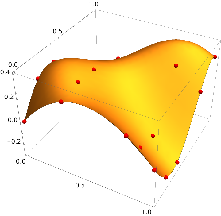 |
With inexact inputs, the result of BezierInterpolatingControlPoints is usually more accurate than using LinearSolve with BernsteinBasis:
| In[9]:= | ![rExact = LinearSolve[
Outer[BernsteinBasis[15, #2, #1] &, Range[16]/17, Range[0, 15]], yl];
xl = N[Range[16]/17]; yl = {2, 1, 2, 3, \[Minus]1, 0, 1, \[Minus]2, 4,
1, 1, \[Minus]3, 0, \[Minus]1, \[Minus]1, 2};
r1 = BezierInterpolatingCoefficients[xl, yl]](https://www.wolframcloud.com/obj/resourcesystem/images/ffd/ffd1599e-8282-4793-b7ab-741577254934/494a44b3d86cdd12.png) |
| Out[9]= |
| In[10]:= |
| Out[10]= |
| In[11]:= |
| Out[11]= |
| In[12]:= |
| Out[12]= |
This work is licensed under a Creative Commons Attribution 4.0 International License