Wolfram Function Repository
Instant-use add-on functions for the Wolfram Language
Function Repository Resource:
Compute the torsion of a curve
ResourceFunction["CurveTorsion"][c,t] computes the torsion of a space curve c parametrized by t. |
Plot the twisted cubic curve:
| In[1]:= |
| Out[1]= | 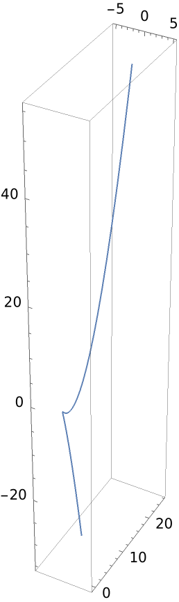 |
Compute the torsion of the twisted cubic curve:
| In[2]:= |
| Out[2]= |
Compute the curvature using the resource function Curvature:
| In[3]:= |
| Out[3]= |
Plot them:
| In[4]:= |
| Out[4]= | 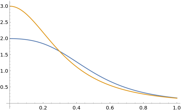 |
For this curve, the torsion and curvature are the same:
| In[5]:= |
| Out[5]= |
| In[6]:= |
| Out[6]= |
Plot of the above results:
| In[7]:= |
| Out[7]= | 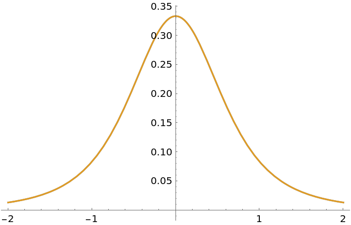 |
A curve that is qualitatively similar to a torus knot:
| In[8]:= |
| Out[8]= |
Plot the curve:
| In[9]:= |
| Out[9]= | 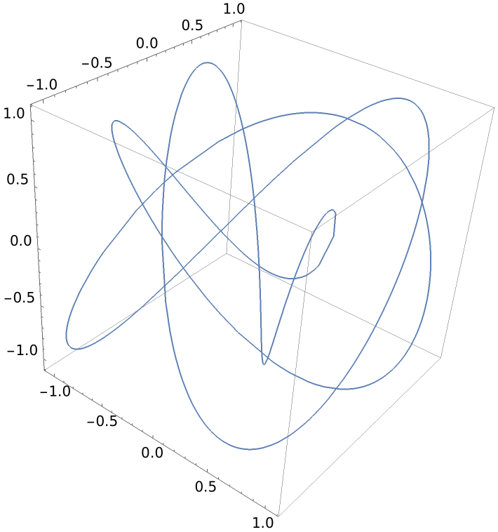 |
Find the torsion:
| In[10]:= |
| Out[10]= |  |
Plot this:
| In[11]:= |
| Out[11]= | 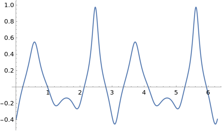 |
Compute the curvature with the resource function Curvature:
| In[12]:= |
| Out[12]= |  |
| In[13]:= |
| Out[13]= | 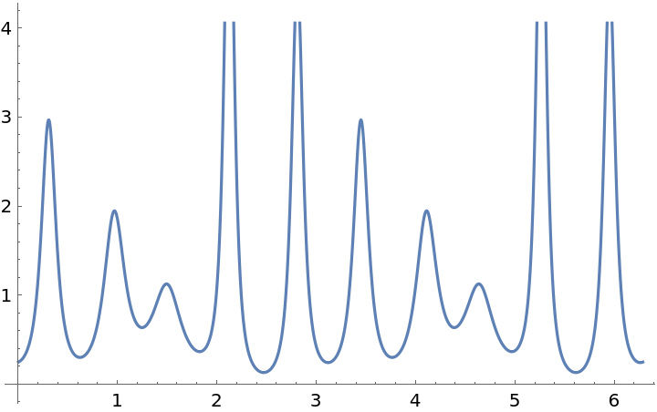 |
Define a conical spiral:
| In[14]:= |
| Out[14]= |
Here is the torsion:
| In[15]:= |
| Out[15]= |
There are other quantities related to torsion. The inverse of the torsion is called the radius of torsion:
| In[16]:= |
| Out[16]= |
The curvature, which can be calculated with the resource function Curvature:
| In[17]:= |
| Out[17]= |
There is also the so-called total curvature:
| In[18]:= |
| Out[18]= |
Definition of a unit speed helix:
| In[19]:= | ![uhelix = {a Cos[t/Sqrt[a^2 + b^2]], a Sin[t/Sqrt[a^2 + b^2]], (b t)/
Sqrt[a^2 + b^2]};](https://www.wolframcloud.com/obj/resourcesystem/images/ff9/ff9aa74a-a6aa-4d88-bdda-9760be172c0e/6bab384b4ca5ef43.png) |
The curvature, via the resource function Curvature:
| In[20]:= |
| Out[20]= |
The torsion:
| In[21]:= |
| Out[21]= |
The relation to the Frenet-Serret system is that the curvature and the torsion are the first two quantities:
| In[22]:= |
| Out[22]= |
This work is licensed under a Creative Commons Attribution 4.0 International License