Details and Options
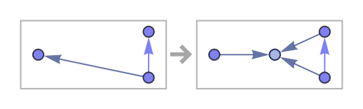
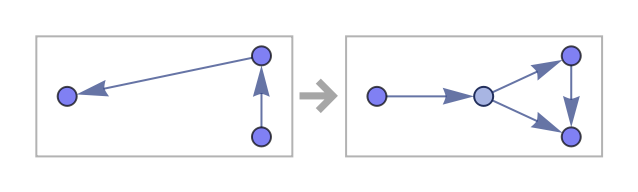
Rules can be a list of the form {rule1,rule2,…} where each of the rulei has the form {{a1,a2,…},{b1,b2,…}, …}→{{u1,u2,…},…}. In this case, the ai etc. can be any expressions, but are assumed to be pattern variables for the purposes of the rule.
Rules of the form <|"PatternRules"→rules|> can be used to specify explicit pattern rules, in which pattern variables must be given as x_, etc., and literals are treated verbatim.
The initial condition init should be of the form {{i1,i2,…},{j1,j2,…},…}.
The initial condition can be
Automatic, in which case the minimum
{{1,1,…},…} initial condition that provides a unification of the rule will be used.
ResourceFunction["WolframModel"][rules,init,t,…] gives results for t complete generations, or fewer if a fixed point is reached earlier.
ResourceFunction["WolframModel"][rules,init,assoc,…] can be used to specify alternative termination criteria. Possible elements in assoc include:
| "MaxEvents" | maximum number of events to allow |
| "MaxGenerations" | maximum number of generations to allow |
| "MaxVertices" | maximum number of hypergraph vertices |
| "MaxEdges" | maximum number of hypergraph edges |
| "MaxVertexDegree" | maximum degree of any vertex |
A generation is defined to end when no more updates can be done without re-updating a node that has already been updated in that generation.
Each generation in effect contains all updates in a single layer in the causal network.
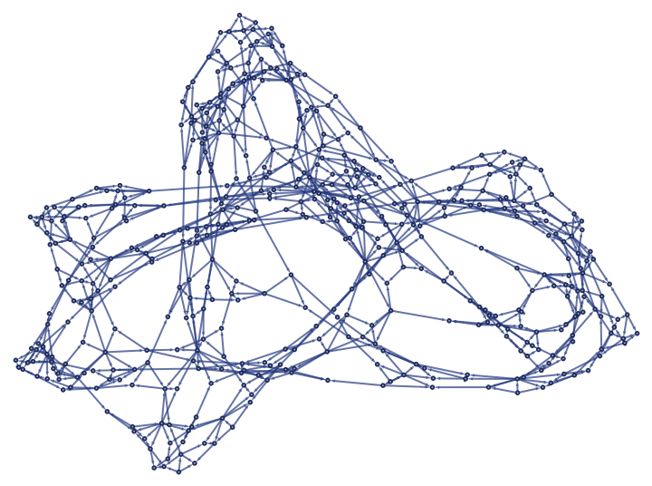
In ResourceFunction["WolframModel"][rules,init,t,prop], possible forms for prop include:
| "EvolutionObject" (default) | the complete evolution object |
| "StatesList" | the list of states for each complete generation |
| "StatesPlotsList" | list of plots of states |
| "FinalState" | the final state only |
| "FinalStatePlot" | plot of the final state |
| "AllEventsStatesList" | the list of all states after all updating events |
| "AllEventsList" | the list of all updating events during the evolution |
| "AllEventsRuleIndices" | list of indices of transformation rules used during the evolution |
| "EventsStatesList" | the list of successive events and states during the evolution |
| "EventsStatesPlotsList" | list of plots of successive states with each event highlighted |
| "AllEventsEdgesList" | the list of all edges in the order they are generated by events |
| "EdgeCreatorEventIndices" | the indices of the updating event that creates each edge |
| "EdgeDestroyerEventIndices" | the indices of the updating event that destroys each edge |
| "VertexCountList" | the list of vertex counts for each complete generation |
| "EdgeCountList" | the list of edge counts for each complete generation |
| "GenerationsCount" | the number of complete and partial generations |
| "GenerationEventsCountList" | the number of events between successive generations |
| "GenerationEventsList" | the list of events between successive generations |
| "EdgeGenerationsList" | which generation each edge is associated with |
| "EventGenerationsList" | which generation each event is associated with |
| "AllEventsCount" | the total number of events in the evolution |
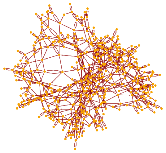
| "CausalGraph" | the causal graph for the evolution |
| "LayeredCausalGraph" | the causal graph rendered in layered form |
| "ExpressionsEventsGraph" | the causal graph that includes both expressions and events as vertices |
| {prop1,prop2,…} | list of results for multiple properties |
ResourceFunction["WolframModel"][rules][state] gives the result of one generation of evolution from state according to rules.
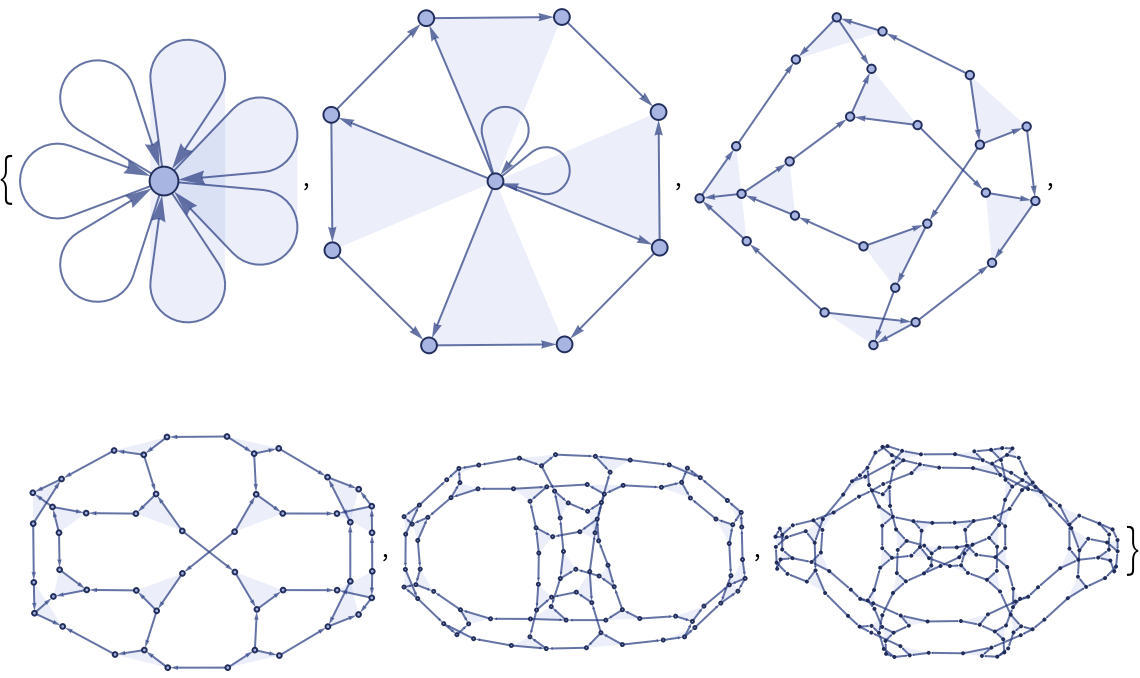
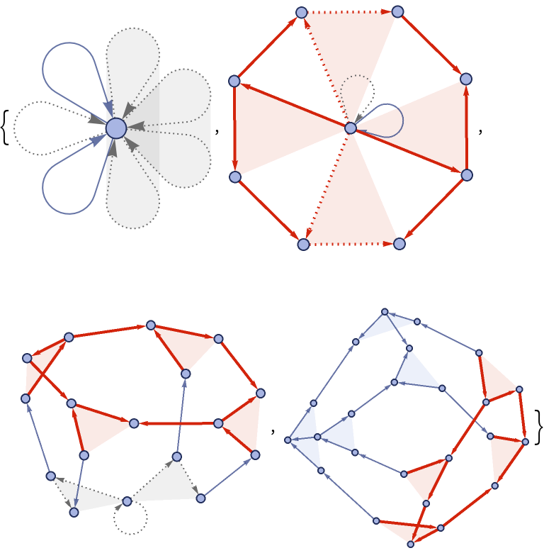
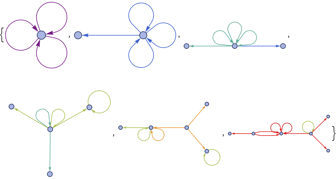
RulePlot[ResourceFunction["WolframModel"][rules]] gives a visual representation of the specified Wolfram model rules.
The property "EventsList" gives specifications of all updating events done on the system. Each is given as the index of the original rule used, as well as the indices of the edges used. These indices can be converted to instantiated edges using "AllEventsEdgesList".
"EventsStatesList" gives pairs of events and the states they produce. The events are specified as a list of edges from "AllEventsEdgesList".
The following options for ResourceFunction["WolframModel"] can be used:
| EventOrderingFunction | Automatic | how to order possible updating events |
| EventSelectionFunction | "GlobalSpacelike" | how to select the rule matches to be instantiated |
| IncludeBoundaryEvents | None | whether to include initial or final events |
| IncludePartialGenerations | Automatic | whether to include incomplete generations |
| Method | Automatic | the method to use ("LowLevel", "Symbolic") |
| TimeConstraint | Infinity | how much CPU time to allow the evolution to run |
| VertexNamingFunction | Automatic | how to name generated elements |
VertexNamingFunction→All renames all vertices to be labeled sequentially starting from 1 , across all generations in the evolution.
VertexNamingFunction→Automatic uses any existing labels, and labels each new vertex with the smallest unallocated integer.
VertexNamingFunction→None uses internal symbol names for new vertices.
Possible settings for IncludeBoundaryEvents include
"Initial",
"Final",
All and
None.
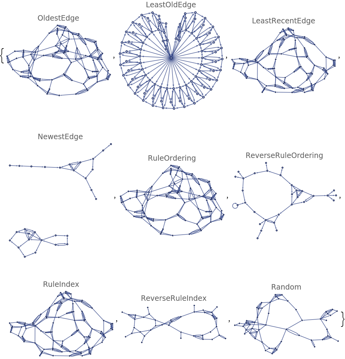
Possible settings for EventOrderingFunction include:
| Automatic | use standard order (least-recent edge, rule ordering, rule index) |
| "Random" | pick the next event at random |
| {ord1,ord2,…} | use the specified sequence of criteria to determine the next event |
With the default setting
EventOrderingFunction→Automatic,
ResourceFunction["WolframModel"] chooses first whatever possible event involves as its newest edge the least recently generated edge. In case of a tie, the permutation of edges closest to the order from the statement of the rule is used. If there is still a tie, then the smallest index rule is used.
Possible ordering criteria:
| "OldestEdge" | sort rule inputs by edge index, and pick the smallest list |
| "LeastOldEdge" | sort rule inputs by edge index, and pick the largest list |
| "LeastRecentEdge" | sort rule inputs by edge index in reverse order, and pick the smallest list |
| "NewestEdge" | sort rule inputs by edge index in reverse order, and pick the largest list |
| "RuleOrdering" | pick the smallest list of edge indices, arranged as in the rule input |
| "ReverseRuleOrdering" | pick the largest list of edge indices, arranged as in the rule input |
| "RuleIndex" | use the earlier rule in a multirule system |
| "ReverseRuleIndex" | use the later rule in a multirule system |
| "Random" | out of events selected by other criteria, pick one uniformly at random |
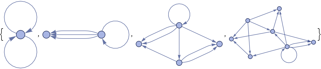
EventSelectionFunction determines the type of the singleway/multiway system to run. Possible values:
| "GlobalSpacelike" | a normal singleway system, expressions are deleted after they are used |
| None | a match-all multiway system that matches spacelike, branchlike and timelike expressions |
See the SetReplace
README for a more detailed documentation.
Install the
SetReplace paclet to get syntax autocompletion, better performance and bleeding-edge functionality.
![evolution = ResourceFunction[
"WolframModel"][{{{1, 1, 2}} -> {{2, 2, 1}, {2, 3, 2}, {1, 2, 3}}, {{1, 2, 1}, {3, 4, 2}} -> {{4, 3, 2}}}, {{1, 1, 1}}, 4]](https://www.wolframcloud.com/obj/resourcesystem/images/f6e/f6eb4e01-15fd-4c52-857b-52f627495c74/5c92532427ccb860.png)
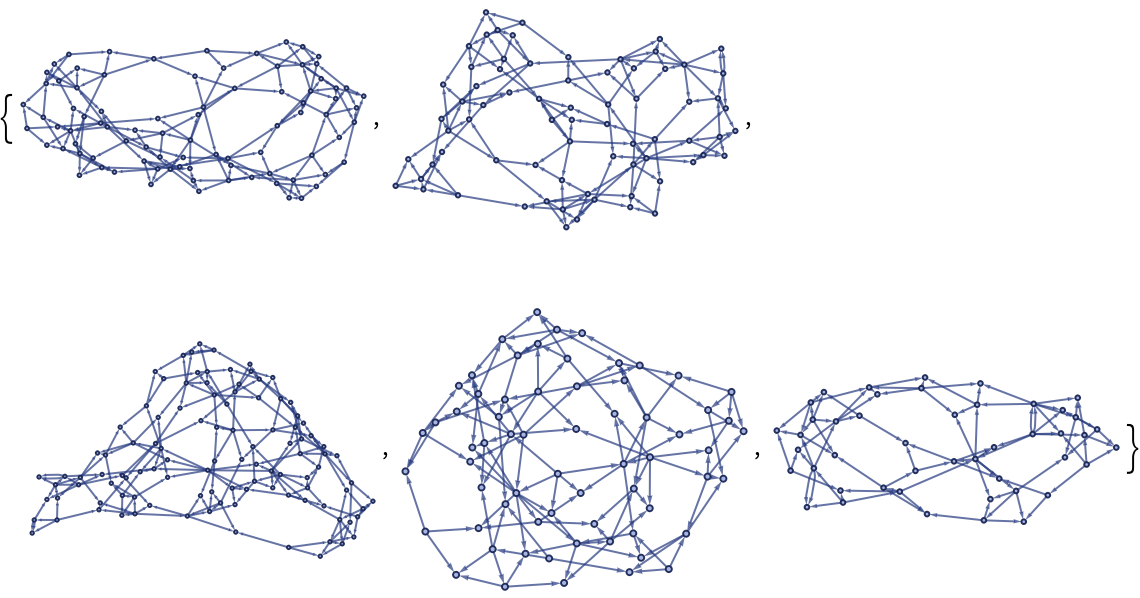
![ResourceFunction[
"WolframModel"][{{1, 2, 3}, {4, 5, 6}, {1, 4}} -> {{2, 7, 8}, {3, 9, 10}, {5, 11, 12}, {6, 13, 14}, {8, 12}, {11, 10}, {13, 7}, {14, 9}}, {{1, 1, 1}, {1, 1, 1}, {1, 1}, {1, 1}, {1, 1}}, 5, "StatesPlotsList"]](https://www.wolframcloud.com/obj/resourcesystem/images/f6e/f6eb4e01-15fd-4c52-857b-52f627495c74/32a66e957503b688.png)
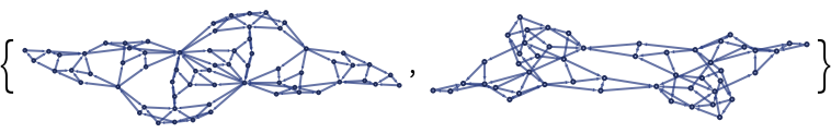
![ResourceFunction[
"WolframModel"][{{1, 2, 3}, {4, 5, 6}, {1, 4}} -> {{2, 7, 8}, {3, 9, 10}, {5, 11, 12}, {6, 13, 14}, {8, 12}, {11, 10}, {13, 7}, {14, 9}}, {{1, 1, 1}, {1, 1, 1}, {1, 1}, {1, 1}, {1, 1}}, 2, "FinalState"]](https://www.wolframcloud.com/obj/resourcesystem/images/f6e/f6eb4e01-15fd-4c52-857b-52f627495c74/7b66b3c99f439cfa.png)
![ResourceFunction[
"WolframModel"][{{1, 2, 3}, {4, 5, 6}, {1, 4}} -> {{2, 7, 8}, {3, 9, 10}, {5, 11, 12}, {6, 13, 14}, {8, 12}, {11, 10}, {13, 7}, {14, 9}}, {{1, 1, 1}, {1, 1, 1}, {1, 1}, {1, 1}, {1, 1}}, 6, "FinalStatePlot"]](https://www.wolframcloud.com/obj/resourcesystem/images/f6e/f6eb4e01-15fd-4c52-857b-52f627495c74/720899c3a75729cf.png)


![ResourceFunction[
"WolframModel"][{{1, 2, 3}, {4, 5, 6}, {1, 4}} -> {{2, 7, 8}, {3, 9, 10}, {5, 11, 12}, {6, 13, 14}, {8, 12}, {11, 10}, {13, 7}, {14, 9}}, {{1, 1, 1}, {1, 1, 1}, {1, 1}, {1, 1}, {1, 1}}, 2, "EventsStatesPlotsList"]](https://www.wolframcloud.com/obj/resourcesystem/images/f6e/f6eb4e01-15fd-4c52-857b-52f627495c74/2cf5582e1b86c200.png)
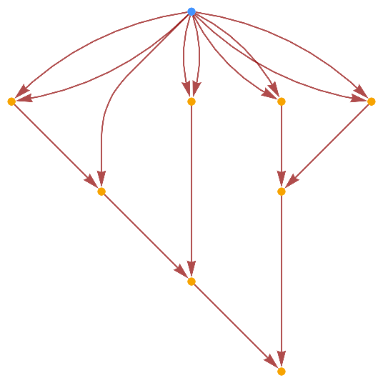
![ResourceFunction[
"WolframModel"][{{1, 2, 3}, {4, 5, 6}, {1, 4}} -> {{3, 7, 8}, {9, 2, 10}, {11, 12, 5}, {13, 14, 6}, {7, 12}, {11, 9}, {13, 10}, {14, 8}}, {{1, 1, 1}, {1, 1, 1}, {1, 1}, {1, 1}, {1, 1}}, 20, "CausalGraph"]](https://www.wolframcloud.com/obj/resourcesystem/images/f6e/f6eb4e01-15fd-4c52-857b-52f627495c74/083c6a1e704278d2.png)
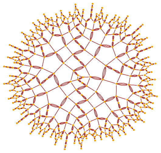
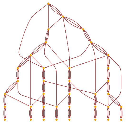
![ResourceFunction[
"WolframModel"][{{1, 2, 3}, {4, 5, 6}, {1, 4}} -> {{3, 7, 8}, {9, 2, 10}, {11, 12, 5}, {13, 14, 6}, {7, 12}, {11, 9}, {13, 10}, {14, 8}}, {{1, 1, 1}, {1, 1, 1}, {1, 1}, {1, 1}, {1, 1}}, 10, "LayeredCausalGraph"]](https://www.wolframcloud.com/obj/resourcesystem/images/f6e/f6eb4e01-15fd-4c52-857b-52f627495c74/70a195c635a2b4a4.png)


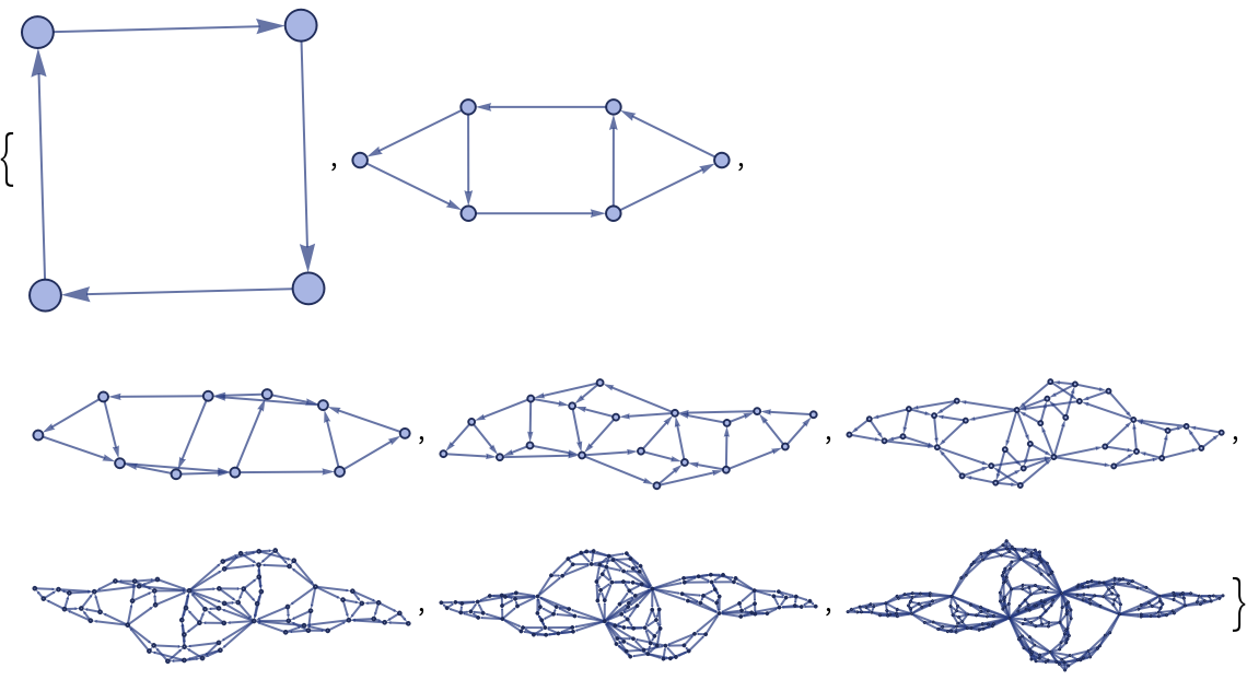
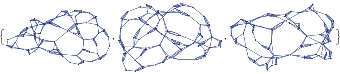
![Table[ResourceFunction[
"WolframModel"][{{x, y}, {x, z}} -> {{x, z}, {x, w}, {y, w}, {z, w}}, {{0, 0}, {0, 0}}, 10, "FinalStatePlot", "EventOrderingFunction" -> "Random"], 5]](https://www.wolframcloud.com/obj/resourcesystem/images/f6e/f6eb4e01-15fd-4c52-857b-52f627495c74/6fa41d921d84c29a.png)

![ResourceFunction["WolframModel"][
ResourceFunction[
"FindCanonicalWolframModel"][{{x, y}, {x, z}} -> {{x, z}, {x, w}, {y, w}, {z, w}}], Automatic, 3, "StatesPlotsList"]](https://www.wolframcloud.com/obj/resourcesystem/images/f6e/f6eb4e01-15fd-4c52-857b-52f627495c74/09735a0ec5bef7f1.png)
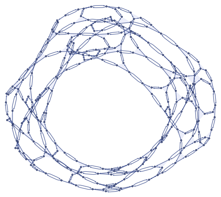
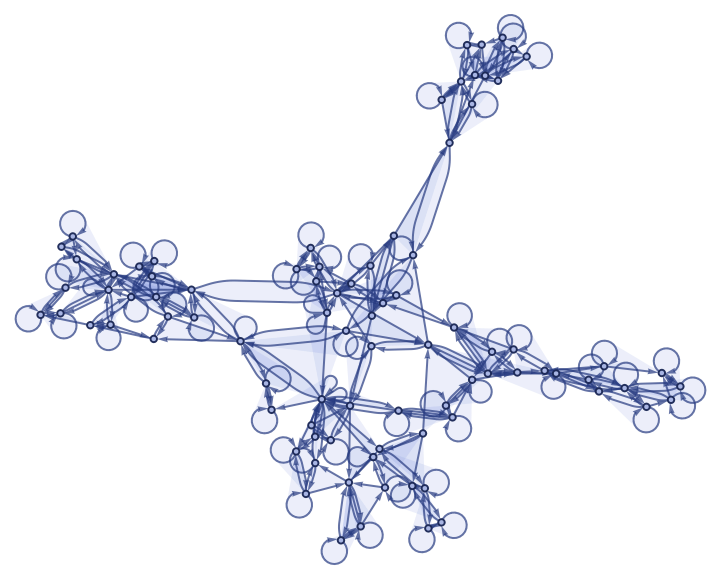
![ResourceFunction[
"WolframModel"][{{1, 2, 3}, {4, 5, 6}, {2, 5}, {5, 2}} -> {{7, 1, 8}, {9, 3, 10}, {11, 4, 12}, {13, 6, 14}, {7, 13}, {13, 7}, {8, 10}, {10, 8}, {9, 11}, {11, 9}, {12, 14}, {14, 12}}, {{1, 2, 3}, {4, 5, 6}, {1, 4}, {4, 1}, {2, 5}, {5, 2}, {3, 6}, {6, 3}}, <|
"MaxVertices" -> 300, "MaxEvents" -> 200|>, "FinalStatePlot"]](https://www.wolframcloud.com/obj/resourcesystem/images/f6e/f6eb4e01-15fd-4c52-857b-52f627495c74/3591efb9585f98ca.png)
![ResourceFunction[
"WolframModel"][{{1, 2, 3}, {4, 5, 6}, {2, 5}, {5, 2}} -> {{7, 1, 8}, {9, 3, 10}, {11, 4, 12}, {13, 6, 14}, {7, 13}, {13, 7}, {8, 10}, {10, 8}, {9, 11}, {11, 9}, {12, 14}, {14, 12}}, {{1, 2, 3}, {4, 5, 6}, {1, 4}, {4, 1}, {2, 5}, {5, 2}, {3, 6}, {6, 3}}, <|
"MaxVertices" -> 300, "MaxEvents" -> 200|>, "FinalStatePlot", "IncludePartialGenerations" -> False]](https://www.wolframcloud.com/obj/resourcesystem/images/f6e/f6eb4e01-15fd-4c52-857b-52f627495c74/0d51e5a5e1b0d4a8.png)
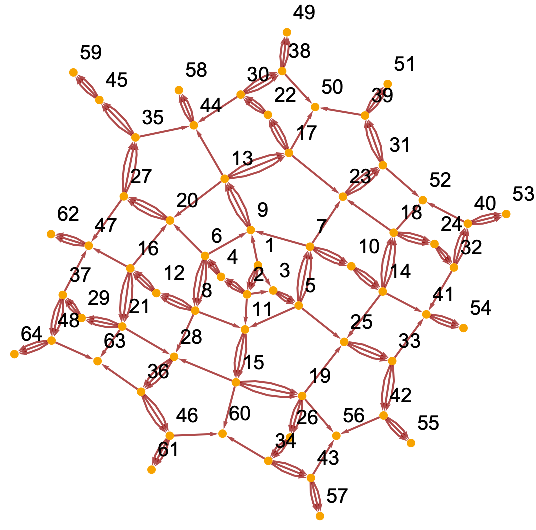
![ResourceFunction[
"WolframModel"][{{1, 2, 3}, {4, 5, 6}, {1, 4}} -> {{3, 7, 8}, {9, 2, 10}, {11, 12, 5}, {13, 14, 6}, {7, 12}, {11, 9}, {13, 10}, {14, 8}}, {{1, 1, 1}, {1, 1, 1}, {1, 1}, {1, 1}, {1, 1}}, 12, "CausalGraph", VertexLabels -> Automatic]](https://www.wolframcloud.com/obj/resourcesystem/images/f6e/f6eb4e01-15fd-4c52-857b-52f627495c74/6aa63bda3b02a16c.png)
![ResourceFunction[
"WolframModel"][{{1, 2, 3}, {4, 5, 6}, {1, 4}} -> {{3, 7, 8}, {9, 2,
10}, {11, 12, 5}, {13, 14, 6}, {7, 12}, {11, 9}, {13, 10}, {14, 8}}, {{1, 1, 1}, {1, 1, 1}, {1, 1}, {1, 1}, {1, 1}}, 12]["CausalGraph", VertexLabels -> Automatic]](https://www.wolframcloud.com/obj/resourcesystem/images/f6e/f6eb4e01-15fd-4c52-857b-52f627495c74/7eddd37430f6da3a.png)
![AbsoluteTiming[
ResourceFunction[
"WolframModel"][{{{0}} -> {{0}, {0}, {0}}, {{0}, {0}, {0}} -> {{0}}}, {{0}}, <|"MaxEvents" -> 30|>, Method -> "LowLevel"]]](https://www.wolframcloud.com/obj/resourcesystem/images/f6e/f6eb4e01-15fd-4c52-857b-52f627495c74/517d083255770c22.png)
![AbsoluteTiming[
ResourceFunction[
"WolframModel"][{{{0}} -> {{0}, {0}, {0}}, {{0}, {0}, {0}} -> {{0}}}, {{0}}, <|"MaxEvents" -> 30|>, Method -> "Symbolic"]]](https://www.wolframcloud.com/obj/resourcesystem/images/f6e/f6eb4e01-15fd-4c52-857b-52f627495c74/7b98bf5565ac465a.png)
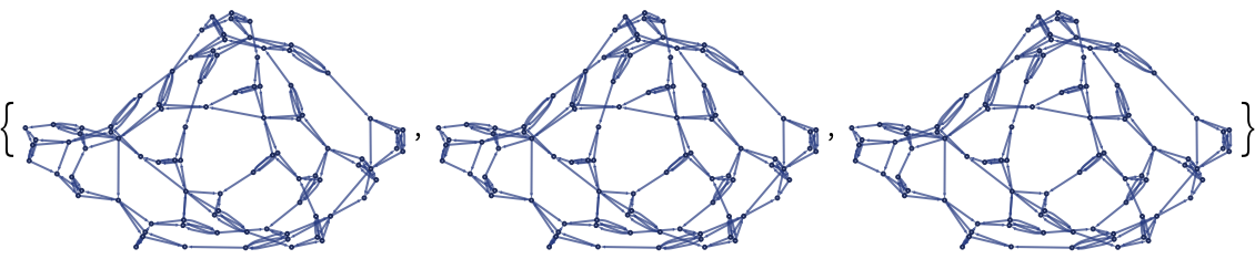
![Table[ResourceFunction[
"WolframModel"][{{{1, 2}, {1, 3}, {1, 4}} -> {{5, 6}, {6, 7}, {7, 5}, {5, 7}, {7, 6}, {6, 5}, {5, 2}, {6, 3}, {7, 4}, {2, 7}, {4, 5}}, {{1, 2}, {1, 3}, {1, 4}, {1, 5}} -> {{2, 3}, {3, 4}}}, {{1,
1}, {1, 1}, {1, 1}}, <|"MaxEvents" -> 30|>, "FinalStatePlot", "EventOrderingFunction" -> "LeastRecentEdge"], 3]](https://www.wolframcloud.com/obj/resourcesystem/images/f6e/f6eb4e01-15fd-4c52-857b-52f627495c74/114ef101f5f0630e.png)
![Table[ResourceFunction[
"WolframModel"][{{{1, 2}, {1, 3}, {1, 4}} -> {{5, 6}, {6, 7}, {7, 5}, {5, 7}, {7, 6}, {6, 5}, {5, 2}, {6, 3}, {7, 4}, {2, 7}, {4, 5}}, {{1, 2}, {1, 3}, {1, 4}, {1, 5}} -> {{2, 3}, {3, 4}}}, {{1,
1}, {1, 1}, {1, 1}}, <|"MaxEvents" -> 30|>, "FinalStatePlot", "EventOrderingFunction" -> {"LeastRecentEdge", "RuleOrdering"}], 3]](https://www.wolframcloud.com/obj/resourcesystem/images/f6e/f6eb4e01-15fd-4c52-857b-52f627495c74/70754a35ed5c3915.png)
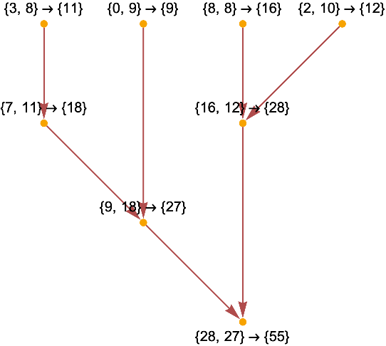
![With[{evolution = ResourceFunction[
"WolframModel"][<|"PatternRules" -> {a_, b_} :> a + b|>, {3, 8, 8,
8, 2, 10, 0, 9, 7}, Infinity]}, With[{causalGraph = evolution["LayeredCausalGraph"]}, Graph[causalGraph, VertexLabels -> Thread[VertexList[causalGraph] -> Map[evolution["AllEventsEdgesList"][[#]] &, Last /@ evolution["AllEventsList"], {2}]]]]]](https://www.wolframcloud.com/obj/resourcesystem/images/f6e/f6eb4e01-15fd-4c52-857b-52f627495c74/46cee67c96fb254e.png)
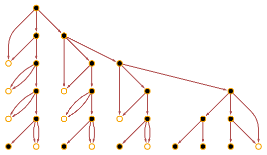
![With[{evolution = ResourceFunction[
"WolframModel"][{{{1, 1, 2}} -> {{2, 2, 1}, {2, 3, 2}, {1, 2, 3}}, {{1, 2, 1}, {3, 4, 2}} -> {{4, 3, 2}}}, {{1, 1, 1}}, 6]},
With[{causalGraph = evolution["LayeredCausalGraph"]}, Graph[causalGraph, VertexStyle -> Thread[VertexList[causalGraph] -> Replace[evolution["AllEventsRuleIndices"], {1 -> Black, 2 -> White}, {1}]], VertexSize -> Medium]]]](https://www.wolframcloud.com/obj/resourcesystem/images/f6e/f6eb4e01-15fd-4c52-857b-52f627495c74/705b9479dc679db5.png)
![With[{evolution = ResourceFunction[
"WolframModel"][{{1, 2}, {1, 3}, {1, 4}} -> {{2, 2}, {3, 2}, {3, 4}, {3, 5}}, {{1, 1}, {1, 1}, {1, 1}}, 5]}, MapThread[
ResourceFunction["WolframModelPlot"][#, EdgeStyle -> #2] &, {evolution["StatesList"], Replace[evolution[
"EdgeGenerationsList"][[#]] & /@ (evolution[
"StateEdgeIndicesAfterEvent", #] &) /@ Prepend[0]@Accumulate@evolution["GenerationEventsCountList"], g_ :> ColorData["Rainbow"][g/5], {2}]}]]](https://www.wolframcloud.com/obj/resourcesystem/images/f6e/f6eb4e01-15fd-4c52-857b-52f627495c74/4c7d15557596aebc.png)
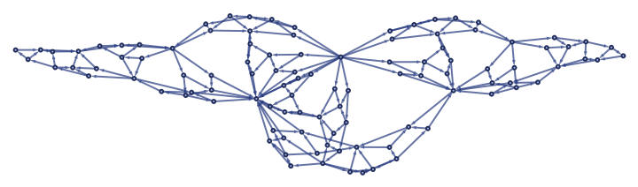
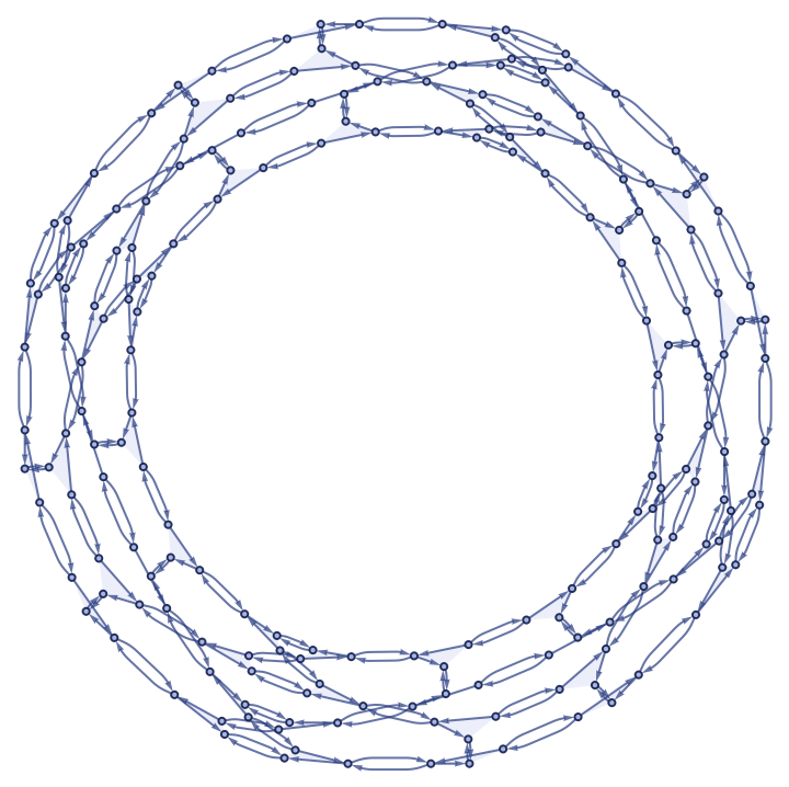
![ResourceFunction[
"WolframModel"][{{1, 2, 3}, {2, 4, 5}} -> {{6, 6, 3}, {2, 6, 2}, {6, 4, 2}, {5, 3, 6}}, {{1, 1, 1}, {1, 1, 1}}, <|
"MaxEvents" -> 10000|>, "FinalStatePlot", "EventOrderingFunction" -> "Random", "IncludePartialGenerations" -> False]](https://www.wolframcloud.com/obj/resourcesystem/images/f6e/f6eb4e01-15fd-4c52-857b-52f627495c74/5e2d7fbecb06ebaa.png)
![ResourceFunction[
"WolframModel"][{{{1, 2}, {1, 3}, {1, 4}} -> {{5, 6}, {6, 7}, {7, 5}, {5, 7}, {7, 6}, {6, 5}, {5, 2}, {6, 3}, {7, 4}, {2, 7}, {4, 5}}, {{1, 2}, {1, 3}, {1, 4}, {1, 5}} -> {{2, 3}, {3, 4}}}, {{1, 1}, {1, 1}, {1, 1}}, <|"MaxEvents" -> 30|>, "EventOrderingFunction" -> {#, "LeastRecentEdge", "RuleOrdering", "RuleIndex"}]["FinalStatePlot", PlotLabel -> #] & /@ {"OldestEdge", "LeastOldEdge", "LeastRecentEdge", "NewestEdge", "RuleOrdering", "ReverseRuleOrdering", "RuleIndex", "ReverseRuleIndex", "Random"}](https://www.wolframcloud.com/obj/resourcesystem/images/f6e/f6eb4e01-15fd-4c52-857b-52f627495c74/08327d1249f59cdc.png)