Wolfram Function Repository
Instant-use add-on functions for the Wolfram Language
Function Repository Resource:
Make a simulation of the Einstein solid
ResourceFunction["EinsteinSolid"][array,steps] makes a simulation of the Einstein solid starting with array and using steps iterations. |
The initial state assigns one quantum to every cell. After about 1,000 steps, the distribution of a thermal equilibrium state and Boltzmann distribution is obtained; it is stable after more steps:
| In[1]:= |
| Out[1]= |  |
Plot the results:
| In[2]:= |
| Out[2]= |  |
| In[3]:= |
| Out[3]= | 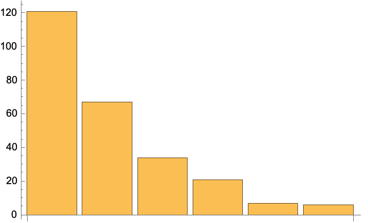 |
After about 20,000 steps, the distribution of energies closely approximates the Boltzmann distribution, and thermal equilibrium is obtained:
| In[4]:= |
| In[5]:= |
| Out[5]= |
The left chart represents instantaneous values m(ε), the right chart represents the mean values given by the canonical distribution ![]() (equal to
(equal to ![]() ) and the red curve represents the fit of the occupancies:
) and the red curve represents the fit of the occupancies:
| In[6]:= |
| Out[6]= | 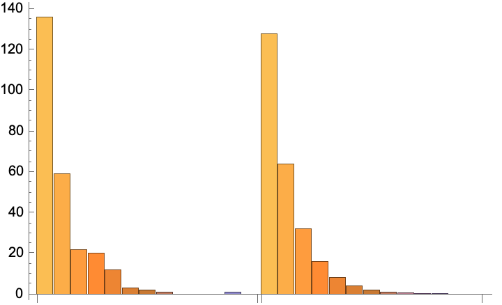 |
Fitting data:
| In[7]:= | ![With[{fit = Fit[Transpose@{Range[0, 12], data}, {2^(-\[Nu])}, \[Nu]]},
Show[RectangleChart[Transpose[{Table[1, {13}], data}]], Plot[Evaluate[fit], {\[Nu], 0, Length[data]}, PlotStyle -> Red, PlotRange -> All], PlotLabel -> Row[List @@ fit, "\[Times]"]]]](https://www.wolframcloud.com/obj/resourcesystem/images/ee7/ee7cd98f-198d-4090-a6ac-85942016780a/1edc2ed4e2e8d016.png) |
| Out[7]= | 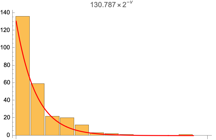 |
The number of points assigned to each cell is the number of quanta possessed by the oscillator (occupancy):
| In[8]:= |
| Out[8]= | 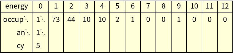 |
Wolfram Language 11.3 (March 2018) or above
This work is licensed under a Creative Commons Attribution 4.0 International License