Wolfram Function Repository
Instant-use add-on functions for the Wolfram Language
Function Repository Resource:
A NetGraph layer implementing focal loss
ResourceFunction["FocalLossLayer"][α,γ] represents a net layer that implements focal loss. |
| "Input" | scalar values between 0 and 1, or arrays of these |
| "Target" | scalar values between 0 and 1, or arrays of these |
| "Loss" | real number |
Create a focal loss layer:
| In[1]:= |
| Out[1]= |  |
Apply it to a given input and target:
| In[2]:= |
| Out[2]= |
Use FocalLossLayer with single probabilities for the input and target:
| In[3]:= |
| Out[4]= |
Apply FocalLossLayer with inputs and targets being matrices of binary-class probabilities:
| In[5]:= |
| Out[6]= |  |
Apply the layer to an input and target:
| In[7]:= |
| Out[7]= |
Use a focal loss layer during training:
| In[8]:= | ![floss = ResourceFunction["FocalLossLayer"][.25, 2];
net = NetInitialize@
NetChain[{8, 1, LogisticSigmoid, PartLayer[1]}, "Input" -> 3, "Output" -> "Boolean"];
trainData = Flatten@Table[{i, j, k} -> (i > j) && (k > i), {i, 10}, {j, 10}, {k,
10}];
result = NetTrain[net, trainData, LossFunction -> floss, TimeGoal -> 3]](https://www.wolframcloud.com/obj/resourcesystem/images/df3/df3512d2-2863-4ef1-8254-d526ca0ba66c/72324695b45c96e7.png) |
| Out[11]= | 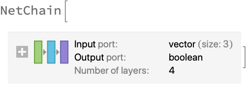 |
| In[12]:= |
| Out[12]= | 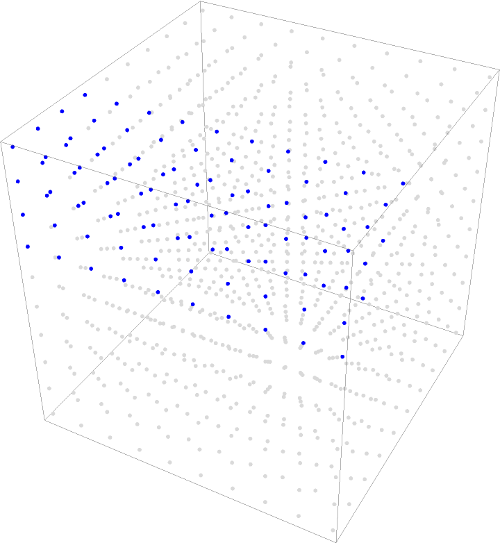 |
Define a FocalLossLayer operating on color images:
| In[13]:= |
| Out[13]= |  |
| In[14]:= | ![DiscretePlot[
rgbloss[<|"Input" -> Image@ConstantArray[{n, n, n}, {10, 10}], "Target" -> Image@ConstantArray[1, {3, 10, 10}]|>], {n, 0, 1, 0.01}, Joined -> False, Filling -> Axis, PlotRange -> Most]](https://www.wolframcloud.com/obj/resourcesystem/images/df3/df3512d2-2863-4ef1-8254-d526ca0ba66c/71a96c2393b75daa.png) |
| Out[14]= | 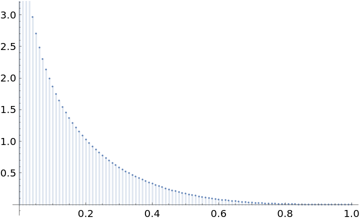 |
Plot a comparison of FocalLossLayer (abbreviated as "FL") and standard CrossEntropy (abbreviated as "CE"). Note that setting γ>0 reduces the relative loss for well-classified examples (pt>.5), thus focusing on the harder examples:
| In[15]:= | ![Clear[fl, vals, exprs];
fl[p_, \[Gamma]_] := -(1 - p)^\[Gamma] Log[p];
vals = {0, .5, 1, 2, 5, 10};
exprs = Table[fl[p, \[Gamma]], {\[Gamma], vals}];
Plot[exprs, {p, 0, 1}, PlotRange -> {{0, 1}, {0, 5}}, PlotLegends -> (HoldForm[\[Gamma] = #] & /@ vals),
FrameTicks -> {{0}~Join~Range[0.2, .8, .2]~Join~{1}, Range[0, 5]},
Frame -> {{True, False}, {True, False}}, FrameLabel -> {"probability of ground truth label", "loss"}, FrameStyle -> 13, PlotRangePadding -> Scaled[.0], ImageMargins -> 5, Epilog -> {Inset[
Style[Column[{Text[
HoldForm[
FL[Subscript[p, t]] = -(1 - Subscript[p, t])^\[Gamma] Log[Subscript[p, t]]]], Text[
HoldForm[CE[Subscript[p, t]] = -Log[Subscript[p, t]]]]}], 16], {.42, 4.1}],
Inset[Style[
\!\(\*UnderscriptBox[\("\<well-classified examples\>"\),
StyleBox["⏞",
FontSize->14,
"NodeID" -> 53]]\), 13, Darker@Gray], {.78, .95}]
}
]](https://www.wolframcloud.com/obj/resourcesystem/images/df3/df3512d2-2863-4ef1-8254-d526ca0ba66c/226120b21b6cf919.png) |
| Out[736]= | 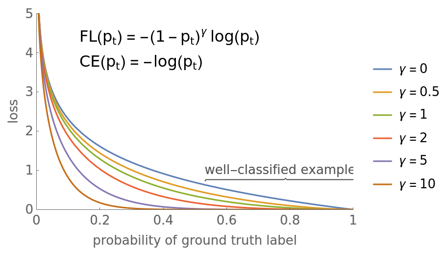 |
This work is licensed under a Creative Commons Attribution 4.0 International License