Wolfram Function Repository
Instant-use add-on functions for the Wolfram Language
Function Repository Resource:
A NetGraph layer implementing cos-dice loss
ResourceFunction["CosDiceLossLayer"][q] represents a net layer that implements cos-dice loss. |
| "Input" | scalar values between 0 and 1, or arrays of these |
| "Target" | scalar values between 0 and 1, or arrays of these |
| "Loss" | real number |
Create a cos-dice loss layer:
| In[1]:= |
| Out[1]= |
And apply it to a given input and target:
| In[2]:= |
| Out[2]= |
Use CosDiceLossLayer with single probabilities:
| In[3]:= |
| Out[4]= |
Apply CosDiceLossLayer with inputs and targets being matrices of binary class probabilities:
| In[5]:= |
| Out[6]= |
Apply the layer to an input and target:
| In[7]:= |
| Out[7]= |
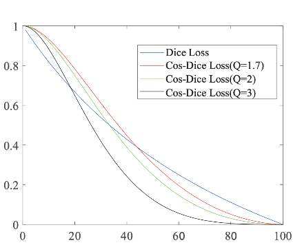
Plot CosDiceLossLayer while varying the q value:
| In[8]:= |
| In[9]:= | ![Manipulate[
l = ResourceFunction["CosDiceLossLayer"][q, "Input" -> enc, "Target" -> enc];
DiscretePlot[
l[<|"Input" -> Image@ConstantArray[n, {64, 64}], "Target" -> Image@ConstantArray[1, {128, 128}]|>], {n, 0, 1, 0.01}, Joined -> True, Filling -> Axis, FillingStyle -> PatternFilling[{"Octagon", Blue}, ImageScaled[1/40]], PlotRange -> {{0, 1}, {0, 1}}, AspectRatio -> 1/2], {{q, 2, "Q"}, 0.1, 10, .5, Appearance -> "Labeled"}, ControlPlacement -> Top]](https://www.wolframcloud.com/obj/resourcesystem/images/dee/deeaf87a-a441-421d-90ed-eabbec913af3/27382c3f3ffd0cf5.png) |
| Out[9]= | 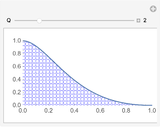 |
This work is licensed under a Creative Commons Attribution 4.0 International License