Wolfram Function Repository
Instant-use add-on functions for the Wolfram Language
Function Repository Resource:
Compute the Balaban J index of an undirected graph or a molecule
ResourceFunction["BalabanJ"][g] computes the Balaban J index of the graph g. | |
ResourceFunction["BalabanJ"][mol] computes the Balaban J index of the Molecule expression mol. |
The Balaban index of a Petersen graph:
| In[1]:= |
| Out[1]= |
Get the same result from GraphData:
| In[2]:= |
| Out[2]= |
Compute the Balaban indices of the order-1 buckyball graph of different classes:
| In[3]:= |
| Out[3]= |
Compute the Balaban indices of two different molecules:
| In[4]:= |
| Out[4]= |
Compute the Balaban index of a named entity:
| In[5]:= |
| Out[5]= |
Compute the Balaban index of the Balaban graph:
| In[6]:= |
| Out[6]= |
By default, hydrogens are ignored in the computation of the Balaban index:
| In[7]:= |
| Out[7]= |
Use IncludeHydrogens→All to account for hydrogens:
| In[8]:= |
| Out[8]= |
A list of straight-chain alkanes:
| In[9]:= | ![alkanes = {Entity["Chemical", "Propane"], Entity["Chemical", "Butane"], Entity["Chemical", "Pentane"], Entity["Chemical", "Hexane"], Entity["Chemical", "Heptane"], Entity["Chemical", "Octane"], Entity["Chemical", "Nonane"], Entity["Chemical", "Decane"], Entity["Chemical", "Undecane"], Entity["Chemical", "Dodecane"]};](https://www.wolframcloud.com/obj/resourcesystem/images/dde/ddef7df2-aea6-4536-bda5-98f8faa39942/2c91ef8b3d7d7901.png) |
Get their corresponding boiling points:
| In[10]:= |
| Out[10]= |
Get their Balaban indices:
| In[11]:= |
| Out[11]= |
The Balaban index is strongly correlated with the logarithm of the boiling point. Visualize the trend:
| In[12]:= |
| Out[12]= | 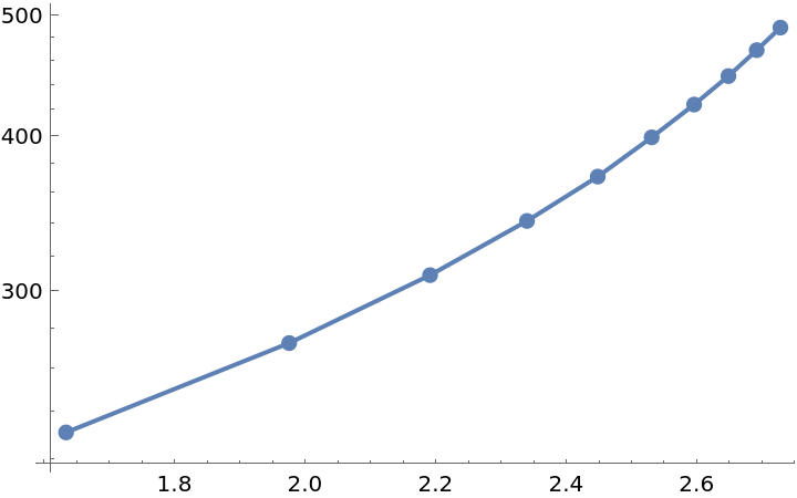 |
Compute the correlation coefficient:
| In[13]:= |
| Out[13]= |
Generate all alkanes with 7 carbon atoms (heptanes) using the resource function AlkaneIsomers:
| In[14]:= |
| Out[14]= | 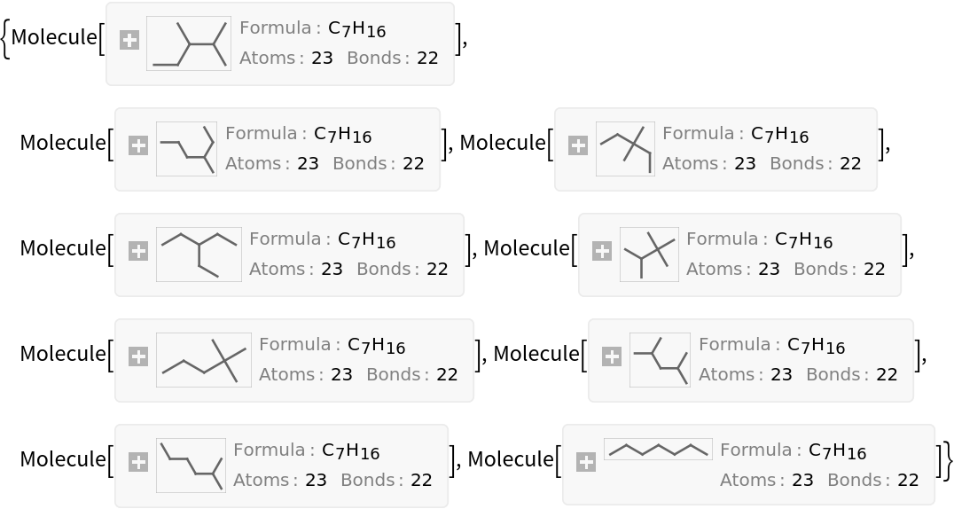 |
The Balaban index can be interpreted as a measure of the amount of branching within an isomeric set of alkanes. Sort the heptane isomers by their Balaban index:
| In[15]:= |
| Out[15]= | 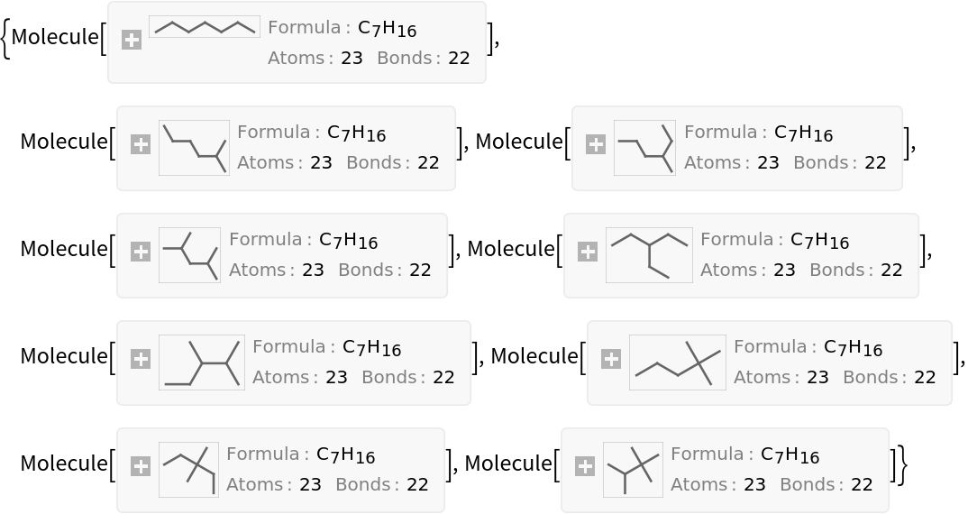 |
The Balaban index of a disconnected graph is 0:
| In[16]:= | ![ResourceFunction["BalabanJ"][\!\(\*
GraphicsBox[
NamespaceBox["NetworkGraphics",
DynamicModuleBox[{Typeset`graph = HoldComplete[
Graph[{1, 2, 3, 4, 5, 6}, {Null, {{1, 3}, {1, 5}, {2, 4}, {2, 6}, {3, 5}, {4, 6}}}, {GraphLayout -> {"VertexLayout" -> "CircularEmbedding",
"PackingLayout" -> None}}]]},
TagBox[GraphicsGroupBox[
GraphicsComplexBox[{{-0.8660254037844389, 0.5000000000000008}, {-0.8660254037844384, -0.4999999999999994}, {3.8285686989269494`*^-16, -1.}, {
0.8660254037844389, -0.5000000000000012}, {
0.8660254037844386, 0.4999999999999993}, {
1.8369701987210297`*^-16, 1.}}, {
{Hue[0.6, 0.7, 0.5], Opacity[0.7],
{Arrowheads[0.], ArrowBox[{1, 3}, 0.02261146496815286]},
{Arrowheads[0.], ArrowBox[{1, 5}, 0.02261146496815286]},
{Arrowheads[0.], ArrowBox[{2, 4}, 0.02261146496815286]},
{Arrowheads[0.], ArrowBox[{2, 6}, 0.02261146496815286]},
{Arrowheads[0.], ArrowBox[{3, 5}, 0.02261146496815286]},
{Arrowheads[0.], ArrowBox[{4, 6}, 0.02261146496815286]}},
{Hue[0.6, 0.2, 0.8], EdgeForm[{GrayLevel[0], Opacity[0.7]}], DiskBox[1, 0.02261146496815286], DiskBox[2, 0.02261146496815286], DiskBox[3, 0.02261146496815286], DiskBox[4, 0.02261146496815286], DiskBox[5, 0.02261146496815286], DiskBox[6, 0.02261146496815286]}}]],
MouseAppearanceTag["NetworkGraphics"]],
AllowKernelInitialization->False]],
DefaultBaseStyle->{"NetworkGraphics", FrontEnd`GraphicsHighlightColor -> Hue[0.8, 1., 0.6]},
FrameTicks->None,
GridLinesStyle->Directive[
GrayLevel[0.5, 0.4]]]\)]](https://www.wolframcloud.com/obj/resourcesystem/images/dde/ddef7df2-aea6-4536-bda5-98f8faa39942/79ffead5b0eafec6.png) |
| Out[16]= |
Wolfram Language 12.3 (May 2021) or above
This work is licensed under a Creative Commons Attribution 4.0 International License