Function Repository Resource:

AsymptoticCurves

Source Notebook

Compute the asymptotic curves of a parameterized surface

Contributed by: Wolfram Staff (original content by Alfred Gray)

ResourceFunction["AsymptoticCurves"][s,{u,v}]

compute the equations for asymptotic curves of a surface s parameterized by variables u and v.

Details and Options

For a regular surface s, an asymptotic curve is a curve c(t) for which the normal curvature vanishes in the direction c'(t).
The differential equation for the asymptotic curves on a surface is e (u')2 + 2f u'v' +g (v')2=0, where e, f and g are coefficients of the second fundamental form.

Examples

Basic Examples (4) 

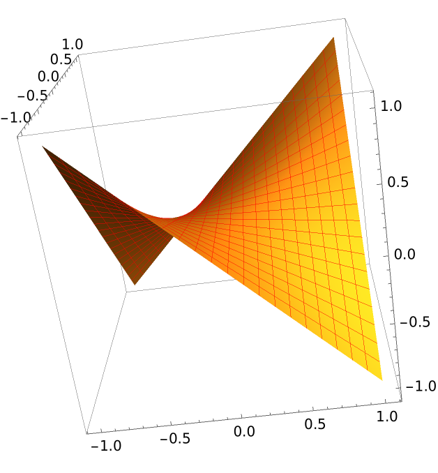
Define a hyperbolic paraboloid:

In[1]:=
hyperbolicparaboloid[u_, v_] := {u, v, u v}

The asymptotic curves are just straight lines:

In[2]:=
ResourceFunction["AsymptoticCurves"][
 hyperbolicparaboloid[u, v], {u, v}]
Out[2]=

The mesh itself represents the asymptotic curves:
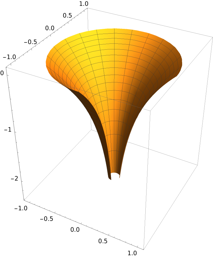
In[3]:=
ParametricPlot3D[hyperbolicparaboloid[u, v], {u, -1, 1}, {v, -1, 1}, Mesh -> {20, 20}, MeshStyle -> Red]
Out[3]=

Define a funnel:

In[4]:=
funnel[a_, b_, c_][u_, v_] := {a v Cos[u], b v Sin[u], c Log[v]}

Plot it:

In[5]:=
ParametricPlot3D[funnel[1, 1, 1][u, v], {u, 0, 3 \[Pi]/2}, {v, .1, 1}]
Out[5]=

Get the equations for asymptotic curves:

In[6]:=
eqs = ResourceFunction["AsymptoticCurves"][
   funnel[1, 1, 1][u, v], {u, v}] // FullSimplify
Out[6]=

Solve the equations:

In[7]:=
Equal @@@ Flatten[{DSolve[eqs[[1]], u[v], v] /. C[1] -> p,
     DSolve[eqs[[2]], u[v], v] /. C[1] -> q} /. u[v] -> \[Theta]] // PowerExpand
Out[7]=

Solve for variables:

In[8]:=
Solve[%, {\[Theta], v}, Reals] // PowerExpand
Out[8]=

Redefine the funnel parameterization in terms of r=ep-q and θ=p+q:

In[9]:=
funnelasym[c_][p_, q_] := {c Exp[p - q] Cos[p + q], -c Exp[p - q] Sin[p + q], c (p - q)}

Plot the asymptotic curves computed in terms of the new coordinates:

In[10]:=
ParametricPlot3D[funnelasym[1][u, v], {u, 0, \[Pi]}, {v, 0, \[Pi]}, PlotPoints -> 50, MaxRecursion -> 3, Mesh -> {30, 30}, MeshStyle -> Red, PlotRange -> {{-4, 2}, {-4, 4}, {-3, 1.3}}]
Out[10]=

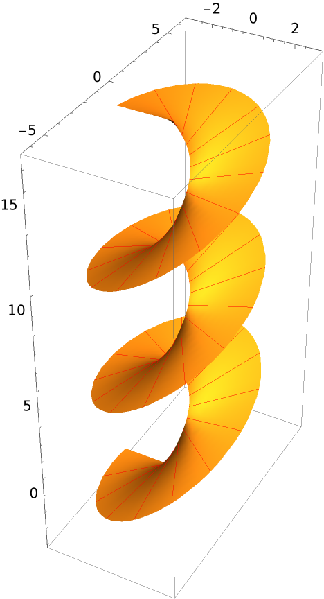
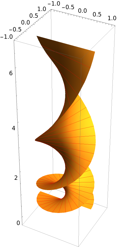
Define the exponentially twisted helicoid:

In[11]:=
exptwist[a_, c_][u_, v_] := {a v Cos[u], a v Sin[u], a Exp[c u]}

Plot the surface:

In[12]:=
ParametricPlot3D[
 exptwist[1, .3][u, v], {u, -\[Pi], 2 \[Pi]}, {v, -1, 1}, PlotPoints -> {24, 12}, Mesh -> {40, 0}, MeshStyle -> Red]
Out[12]=

The asymptotic curve equations:

In[13]:=
eqs = ResourceFunction["AsymptoticCurves"][
  exptwist[a, c][u, v], {u, v}]
Out[13]=

The asymptotic curve solutions:

In[14]:=
{DSolve[eqs[[1]], u[v], v] /. C[1] -> p, DSolve[eqs[[2]], u[v], v] /. C[1] -> q} // Flatten
Out[14]=

Solve for parameters:

In[15]:=
Solve[{u[v] == p, u[v] == q + (2 Log[v])/c} /. u[v] -> \[Theta], {\[Theta], v}, Reals]
Out[15]=

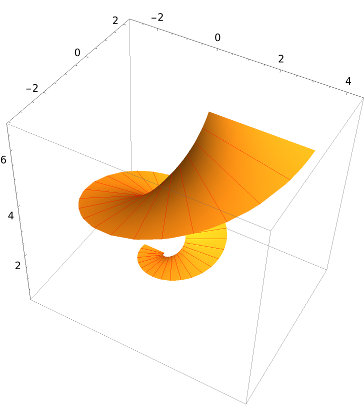
Redefine the parameterization in terms of r =ec(p-q) and θ=p:

In[16]:=
exptwistasym[a_, c_][p_, q_] := a {Exp[1/2 c (p - q)] Cos[p], Exp[1/2 c (p - q)] Sin[p], Exp[c p]}

Plot the asymptotic curves on the exponentially twisted helicoid:

In[17]:=
ParametricPlot3D[
 exptwistasym[1, .3][p, q], {p, -\[Pi], 2 \[Pi]}, {q, -\[Pi], 2 \[Pi]}, PlotPoints -> {36, 12}, PlotRange -> All, Mesh -> {40, 0},
  MeshStyle -> Red]
Out[17]=

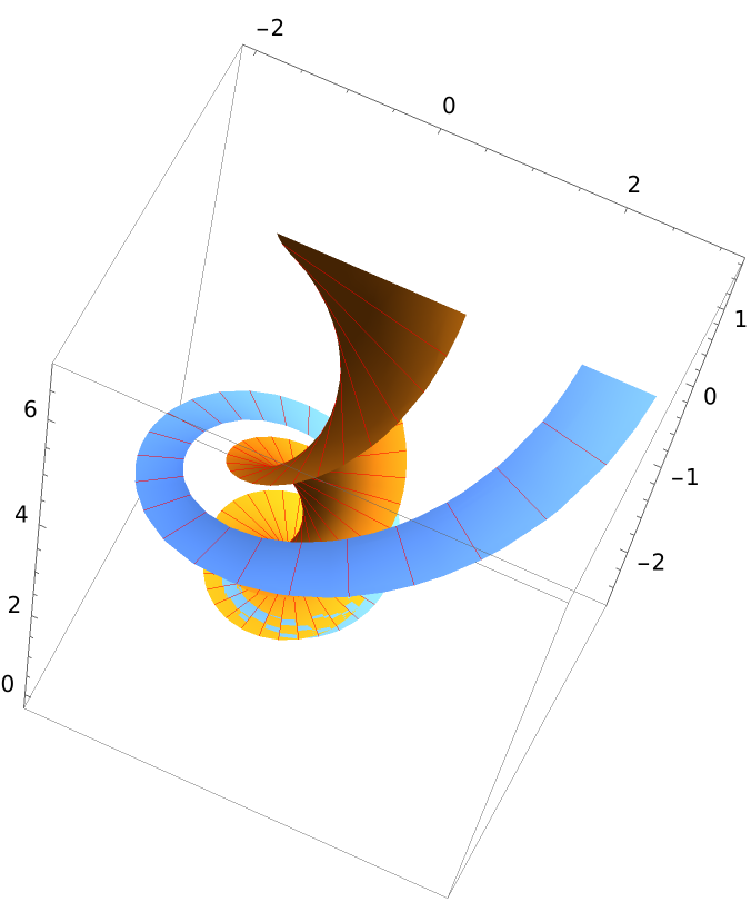
Superimpose both the surface and its asymptotic curves:

In[18]:=
ParametricPlot3D[
 Evaluate[{exptwist[1, .3][u, v], exptwistasym[1, .3][u, v]}], {u, -\[Pi], 2 \[Pi]}, {v, -1, 1}, PlotPoints -> {24, 12}, Mesh -> {40, 0}, MeshStyle -> Red]
Out[18]=

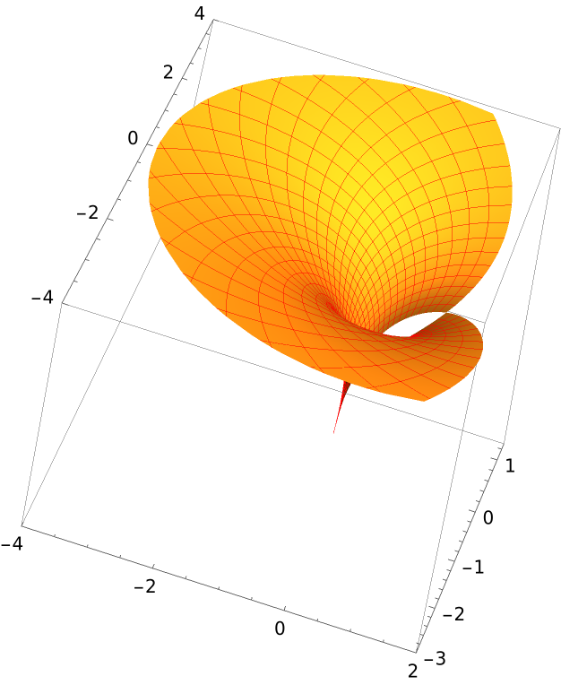
Define a wrinkled surface:

In[19]:=
wrinkles[a_][u_, v_] := {u, v, a (u/v + v/u)}

Plot the surface:

In[20]:=
ParametricPlot3D[wrinkles[0.05][u, v], {u, -1, 1}, {v, -1, 1}]
Out[20]=

Get the equations for asymptotic curves:

In[21]:=
ResourceFunction["AsymptoticCurves"][wrinkles[a][u, v], {u, v}]
Out[21]=

Solve the equations:

In[22]:=
eqs = Equal @@@ Flatten[{DSolve[Derivative[1][u][v] == u[v]^3/v^3, u[v], v] /. C[1] -> q,
      DSolve[Derivative[1][u][v] == u[v]/v, u[v], v] /. C[1] -> p} /. u[v] -> u] // PowerExpand
Out[22]=

Solve for variables:

In[23]:=
{Solve[{eqs[[1]], eqs[[3]]}, {p, q}], Solve[{eqs[[2]], eqs[[3]]}, {p, q}]} // Apart
Out[23]=

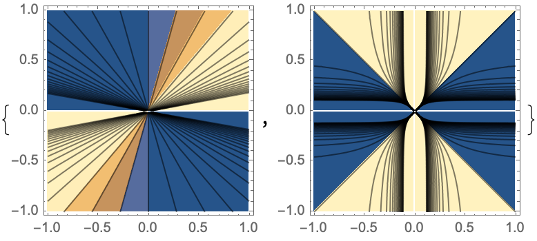
A way to visualize the curves using ContourPlot:

In[24]:=
ContourPlot[#, {x, -1, 1}, {y, -1, 1}, Contours -> 40, ClippingStyle -> Automatic, ColorFunctionScaling -> False] & /@ {x/
   y, 1/x^2 - 1/y^2}
Out[24]=

Properties and Relations (7) 

Define an elliptic helicoid:

In[25]:=
helicoid[a_, b_, c_][u_, v_] := {a v Cos[u], b v Sin[u], c u}

The inner and outer edges of the elliptical helicoid are helices:

In[26]:=
he = helicoid[1, 2, 1];
 ParametricPlot3D[he[u, v], {u, -\[Pi], 5 \[Pi]}, {v, 1/3, 3},
    PlotPoints -> {80, 10}, Mesh -> {40, 0}, MeshStyle -> Red]
Out[26]=

Get the asymptotic curve equation:

In[27]:=
ResourceFunction["AsymptoticCurves"][helicoid[1, 2, 1][u, v], {u, v}]
Out[27]=

For the coefficients of the second fundamental form, only the middle one, f, is nonzero:

In[28]:=
ResourceFunction["SecondFundamentalFormCoefficients"][
 helicoid[1, 2, 1][u, v], {u, v}]
Out[28]=

Now, verify an instance of the Beltrami-Enneper theorem, starting with the Gaussian curvature:

In[29]:=
ResourceFunction["GaussianCurvature"][helicoid[a, b, c][u, v], {u, v}]
Out[29]=

Take a helix that is contained in the helicoid:

In[30]:=
helix[a_, b_, c_][t_] := {a Cos[t], b Sin[t], c t}

Subtract the square of the torsion to give the same expression as shown previously, verifying the identity:

In[31]:=
FullSimplify[-ResourceFunction["CurveTorsion"][helix[a v, b v, c][u], u]^2 /. Abs[e_] -> e]
Out[31]=

Publisher

Enrique Zeleny

Version History

  • 1.0.0 – 30 July 2020

Source Metadata

Related Resources

License Information