Basic Examples (4)
Generate Ω1,com(t) which will be A(t):
Generate Ω1(t):
Generate Ω2,com(t):
Generate Ω2,com(t) while holding the commutation form:
Check whether it is the same as 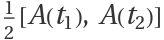 :
:
Do the commutation operation:
Do the commutation operation for Dot as the operation:
Do the commutation operation for Composition as the operation:
Generate Ω2(t):
Applications (27)
H(t)=f(t)(eⅈ ta+e-ⅈ ta†)
Define a time-dependent Hamiltonian as H(t)=f(t)(eⅈ ta+e-ⅈ ta†) with[a,a†]=1 where a (a†) is the annihilation (creation) operator:
The Hamiltonian above is expressed in the interaction picture; see Sec. 4.1.1 of the preprint (arXiv:0810.5488) for details. To avoid any conflict, we shall use formal symbol of t for the time.
Define the variables within the non-commutative algebra together with their corresponding commutation relations:
Since in the Magnus series, there are many time-dependent terms that are only scalar variables, define corresponding non-commutative algebra and Gröbner basis for given n (where we needs to specify what are scalar variables for a given n):
For scalar variables in above definitions, we use the same format as in the Magnus series defined in the previous section.
A function that simplifies and reduces the non-commutative polynomial of the annihilation and creation operators:
We use Nest with ReleaseHold since the Magnus terms defined in the previous section are expressed in the hold commutator form.
As noted earlier, we chose a Hamiltonian that does not commute at different times. Show the Hamiltonian at different times do not commute:
Show[H(t1),[H(t2),H(t3)]]=0:
Find commutation term [H(t1),H(t2)] in the second term of Magnus expansion 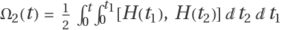 :
:
Find commutation term, [H(t1),[H(t2),H(t3)]], in the third term of Magnus expansion  :
:
It is interesting that the third them and so on are all zero. Therefore, only first and 2nd terms contribute to the exponential:
 which can be rewritten as
U(t)=Exp[-ⅈ (α a+α*a†)-ⅈ β]
with
which can be rewritten as
U(t)=Exp[-ⅈ (α a+α*a†)-ⅈ β]
with 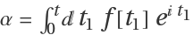 and
and  :
:
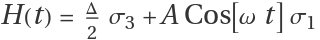
H(t)=f1(t) σ1+f2(t) σ2+f3(t) σ3
Define a time-dependent Hamiltonian as H(t)=f1(t) σ1+f2(t) σ2+f3(t) σ3 with σ1 the Pauli-X, σ2 the Pauli-Y, and σ3 the Pauli-Z:
Define the variables within the non-commutative algebra together with their corresponding commutation relations:
Since in the Magnus series, there are many time-dependent terms that are only scalar variables, define corresponding non-commutative algebra and Gröbner basis for given n (where we needs to specify what are scalar variables for a given n):
A function that simplifies and reduces the non-commutative polynomial of Pauli matrices:
As noted earlier, we chose a Hamiltonian that does not commute at different times. Show the Hamiltonian at different times do not commute:
In above code, we have applied NonCommutativePolynomialReduce two times to take care of all reductions (note the difference in the order of variables):
Define the Hamiltonian as 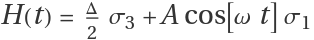 :
:
Define corresponding algebra and Groebner Basis:
Define a function to simplify corresponding polynomials:
Calculate {Ω1(t),Ω2(t),Ω3(t),Ω4(t)} and then collect them by Pauli matrix terms:
For each term, find the coefficient for Pauli matrices (keep in mind that we will have only linear terms):
Now let's repeat the same process, but this time assigning explicit values to Pauli matrics and doing the commutation/dot calculations:
Ω1To4Manual=a1σ1+a2σ2+a3σ3
Note ai=Tr[σi.Ω1To4Manual]/2. One can calculate it and compare with the previous result:
As expected, the coefficients in front of Pauli matrices are the same the ones we obtained from non - commutative algebraic calculations.
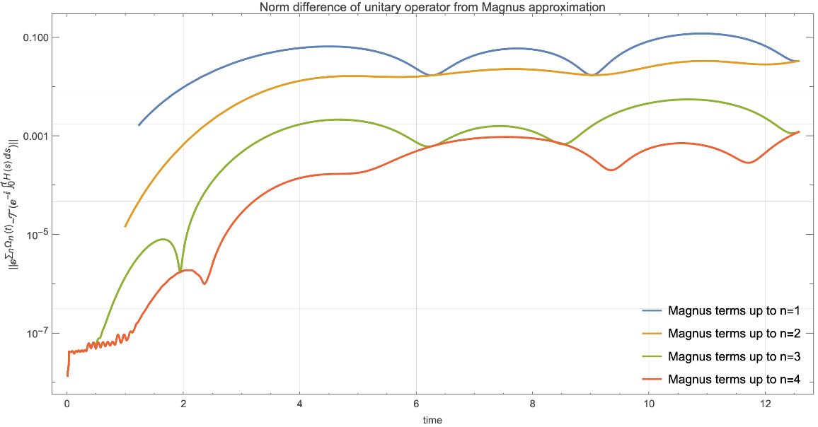
Some numerical exploration. To find approximation to unitary operator determined by H(t), calculate {-ⅈ Ω1(t),(-ⅈ)2Ω2(t),(-ⅈ)3Ω3(t),(-ⅈ)4Ω4(t)}:
Calculate the unitary operator:
Calculate {Ω1(t),∑n=12Ωn(t),∑n=13Ωn(t),∑n=14Ωn(t)}:
Calculate ⅇ∑nΩn(t) and compare it with the solution  :
:
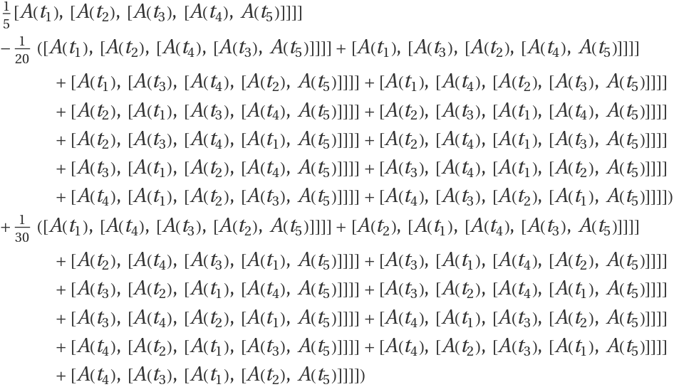
![ResourceFunction[
"MagnusTerms", ResourceSystemBase -> "https://www.wolframcloud.com/obj/resourcesystem/api/1.0"][\[FormalCapitalA], 3] - (1/3 Commutator[\[FormalCapitalA][Subscript[\[FormalT], 1]], Commutator[\[FormalCapitalA][Subscript[\[FormalT], 2]], \[FormalCapitalA][Subscript[\[FormalT], 3]]]] - 1/6 Commutator[\[FormalCapitalA][Subscript[\[FormalT], 2]], Commutator[\[FormalCapitalA][Subscript[\[FormalT], 1]], \[FormalCapitalA][Subscript[\[FormalT], 3]]]]) // NonCommutativeExpand](https://www.wolframcloud.com/obj/resourcesystem/images/d80/d80893ba-51a3-4140-a5a3-ccfb94fb8366/601a3e0b952d2afc.png)

![ResourceFunction[
"MagnusTerms", ResourceSystemBase -> "https://www.wolframcloud.com/obj/resourcesystem/api/1.0"][\[FormalCapitalA], 4] - (1/4 Commutator[\[FormalCapitalA][Subscript[\[FormalT], 1]], Commutator[\[FormalCapitalA][Subscript[\[FormalT], 2]], Commutator[\[FormalCapitalA][Subscript[\[FormalT], 3]], \[FormalCapitalA][Subscript[\[FormalT], 4]]]]] - 1/12 Commutator[\[FormalCapitalA][Subscript[\[FormalT], 1]], Commutator[\[FormalCapitalA][Subscript[\[FormalT], 3]], Commutator[\[FormalCapitalA][Subscript[\[FormalT], 2]], \[FormalCapitalA][Subscript[\[FormalT], 4]]]]] - 1/12 Commutator[\[FormalCapitalA][Subscript[\[FormalT], 2]], Commutator[\[FormalCapitalA][Subscript[\[FormalT], 1]], Commutator[\[FormalCapitalA][Subscript[\[FormalT], 3]], \[FormalCapitalA][Subscript[\[FormalT], 4]]]]] - 1/12 Commutator[\[FormalCapitalA][Subscript[\[FormalT], 2]], Commutator[\[FormalCapitalA][Subscript[\[FormalT], 3]], Commutator[\[FormalCapitalA][Subscript[\[FormalT], 1]], \[FormalCapitalA][Subscript[\[FormalT], 4]]]]] - 1/12 Commutator[\[FormalCapitalA][Subscript[\[FormalT], 3]], Commutator[\[FormalCapitalA][Subscript[\[FormalT], 1]], Commutator[\[FormalCapitalA][Subscript[\[FormalT], 2]], \[FormalCapitalA][Subscript[\[FormalT], 4]]]]] + 1/12 Commutator[\[FormalCapitalA][Subscript[\[FormalT], 3]], Commutator[\[FormalCapitalA][Subscript[\[FormalT], 2]], Commutator[\[FormalCapitalA][Subscript[\[FormalT], 1]], \[FormalCapitalA][Subscript[\[FormalT], 4]]]]]) // NonCommutativeExpand](https://www.wolframcloud.com/obj/resourcesystem/images/d80/d80893ba-51a3-4140-a5a3-ccfb94fb8366/645afff63aeae9b4.png)

 :
:![(* Evaluate this cell to get the example input *) CloudGet["https://www.wolframcloud.com/obj/a89e31eb-03f4-4711-9296-91b19a42d00c"]](https://www.wolframcloud.com/obj/resourcesystem/images/d80/d80893ba-51a3-4140-a5a3-ccfb94fb8366/15b6e61ed0d3e55b.png)
![ClearAll[vars1, rel1]
vars1 = {\[FormalA], SuperDagger[\[FormalA]]};
rel1 = {Commutator[\[FormalA], SuperDagger[\[FormalA]]] - 1};](https://www.wolframcloud.com/obj/resourcesystem/images/d80/d80893ba-51a3-4140-a5a3-ccfb94fb8366/45edfce39ac46f17.png)
![ClearAll[alg1, gb1]
alg1[n_] := NonCommutativeAlgebra[<|
"ScalarVariables" -> Flatten[{#, f[#]} & /@ Table[Subscript[\[FormalT], i], {i, n}]]|>];
gb1[n_] := NonCommutativeGroebnerBasis[rel1, vars1, alg1[n]]](https://www.wolframcloud.com/obj/resourcesystem/images/d80/d80893ba-51a3-4140-a5a3-ccfb94fb8366/66561d08d6652cc2.png)
![ClearAll[vars2, rel2]
vars2 = Table[Subscript[\[Sigma], j], {j, 3}];
rel2 = Table[
Subscript[\[Sigma], i] ** Subscript[\[Sigma], j] - KroneckerDelta[i, j] - I Sum[LeviCivitaTensor[3][[i, j, k]] Subscript[\[Sigma], k], {k, 3}], {i, 3}, {j, 3}] // Flatten](https://www.wolframcloud.com/obj/resourcesystem/images/d80/d80893ba-51a3-4140-a5a3-ccfb94fb8366/6bfdb171f51c3a6e.png)
![ClearAll[alg2, gb2]
alg2[n_] := NonCommutativeAlgebra[<|
"ScalarVariables" -> Join[Flatten[
Table[Subscript[f, j][Subscript[\[FormalT], i]], {j, 3}, {i, n}]],
Table[Subscript[\[FormalT], i], {i, n}]]|>];
gb2[n_] := NonCommutativeGroebnerBasis[rel2, vars2, alg2[n]]](https://www.wolframcloud.com/obj/resourcesystem/images/d80/d80893ba-51a3-4140-a5a3-ccfb94fb8366/5dfdc137caf457ba.png)
![ClearAll[reduceF2]
reduceF2[exp_, n_] := NonCommutativePolynomialReduce[
NonCommutativePolynomialReduce[exp, gb2[n], vars2, alg2[n]][[-1]], gb2[n], Reverse@vars2, alg2[n]][[-1]]](https://www.wolframcloud.com/obj/resourcesystem/images/d80/d80893ba-51a3-4140-a5a3-ccfb94fb8366/5923462c96f57028.png)


![ClearAll[vars2, rel2]
vars2 = Table[Subscript[\[Sigma], j], {j, 3}];
rel2 = Table[
Subscript[\[Sigma], i] ** Subscript[\[Sigma], j] - KroneckerDelta[i, j] - I Sum[LeviCivitaTensor[3][[i, j, k]] Subscript[\[Sigma], k], {k, 3}], {i, 3}, {j, 3}] // Flatten](https://www.wolframcloud.com/obj/resourcesystem/images/d80/d80893ba-51a3-4140-a5a3-ccfb94fb8366/0ed76b19e125ad66.png)
![ClearAll[alg3]
alg3[n_] := NonCommutativeAlgebra[<|
"ScalarVariables" -> Join[{\[CapitalDelta], A, \[Omega]}, Table[Subscript[\[FormalT], i], {i, n}]]|>];
gb3[n_] := NonCommutativeGroebnerBasis[rel2, vars2, alg3[n]]](https://www.wolframcloud.com/obj/resourcesystem/images/d80/d80893ba-51a3-4140-a5a3-ccfb94fb8366/1d4dfcf6f17173c0.png)
![ClearAll[reduceF3]
reduceF3[exp_, n_] := NonCommutativePolynomialReduce[
NonCommutativePolynomialReduce[exp, gb3[n], vars2, alg3[n]][[-1]], gb3[n], Reverse@vars2, alg3[n]][[-1]]](https://www.wolframcloud.com/obj/resourcesystem/images/d80/d80893ba-51a3-4140-a5a3-ccfb94fb8366/1772994115028a9b.png)
![\[CapitalOmega]1To4 = NonCommutativeCollect[FullSimplify@#, vars2, NonCommutativeAlgebra[<|
"ScalarVariables" -> {\[Omega], \[FormalCapitalT], A, \[CapitalDelta]}|>]] & /@ Table[ResourceFunction[
"MagnusTerms", ResourceSystemBase -> "https://www.wolframcloud.com/obj/resourcesystem/api/1.0"][h3, n, reduceF3[#, n] &, "TimeIntegration" -> True], {n, 4}]](https://www.wolframcloud.com/obj/resourcesystem/images/d80/d80893ba-51a3-4140-a5a3-ccfb94fb8366/51cbfe06bb59a954.png)


![ham = (\[CapitalDelta]/2 PauliMatrix[3] + A Cos[\[Omega] t] PauliMatrix[
1] /. {A -> .2, \[CapitalDelta] -> .1, \[Omega] -> 1});
u = NDSolveValue[{\[FormalU]'[
t] == -I ham . \[FormalU][t], \[FormalU][0] == IdentityMatrix[2]}, \[FormalU], {t, 0, tf = 4 \[Pi]}]](https://www.wolframcloud.com/obj/resourcesystem/images/d80/d80893ba-51a3-4140-a5a3-ccfb94fb8366/13dad76a458d4abf.png)
![Legended[
Show[Table[
LogPlot[Norm[
MatrixExp[\[CapitalOmega]n[[j]]] - u[\[FormalCapitalT]]], {\[FormalCapitalT], 10^-3, tf}, PlotStyle -> ColorData[97][j]], {j, 4}], PlotRange -> All, GridLines -> Automatic, PlotLabel -> "Norm difference of unitary operator from Magnus approximation", AspectRatio -> 1/2, Frame -> True, FrameLabel -> {"time", "||\!\(\*SuperscriptBox[\(\[ExponentialE]\), \(\*SubscriptBox[\(\[Sum]\), \(n\)]\*SubscriptBox[\(\[CapitalOmega]\), \(n\)] \((t)\)\)]\)-\[ScriptCapitalT](\!\(\*SuperscriptBox[\(\[ExponentialE]\), \(\(-\[ImaginaryI]\)\\\ \(\*SubsuperscriptBox[\(\[Integral]\), \(0\), \(t\)]H \((s)\) \[DifferentialD]s\)\)]\))||"}, ImageSize -> 800], Placed[LineLegend[Table[ColorData[97][j], {j, 4}], Table["Magnus terms up to n=" <> ToString[j], {j, 4}]], {Right, Bottom}]]](https://www.wolframcloud.com/obj/resourcesystem/images/d80/d80893ba-51a3-4140-a5a3-ccfb94fb8366/3150506e13dd6859.png)