Function Repository Resource:

NormalCurvature

Compute the normal curvature of a curve on a surface

Contributed by: Wolfram Staff (original content by Alfred Gray)

ResourceFunction["NormalCurvature"][s,c,{u,v},t]

computes the normal curvature of the plane curve c with respect to variable t over the surface s parameterized by u and v.

Details and Options

The normal curvature κ_n(v_p) measures how a regular surface M bends in the direction v_p. This quantity is the curvature of the resulting plane curve from the intersection of M with a plane passing through a point p, with tangent v and normal

, being perpendicular to M.

The normal curvature can be defined as

, where

is the unit normal.

The maximum and minimum values of the normal curvature are the principal curvatures.

The normal curvature κ_n in direction φ is given by the Euler curvature formula κ_n=κ₁cos²φ+κ₂sin²φ, where κ₁ and κ₂ are the principal curvatures.

Examples

Basic Examples (2)

A sphere:

In[1]:=

$sphere[a_][u_, v_] := a {Cos[u] Cos[v], Cos[v] Sin[u], Sin[v]}$

Normal curvature of the sphere:

In[2]:=

In[3]:=

A hyperbolic paraboloid:

In[4]:=

$hp = {u, v, -u^2 + v^2/3};$

A normal section of the hyperbolic paraboloid:

In[5]:=

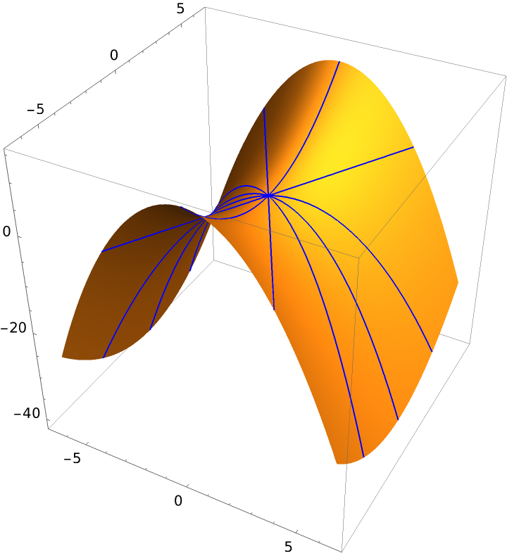
$hpc\[CurlyPhi][\[CurlyPhi]_][ t_] := {u Cos[\[CurlyPhi]], v Sin[\[CurlyPhi]], -(u Cos[\[CurlyPhi]])^2 + (v Sin[\[CurlyPhi]])^2/3} /. {u -> t, v -> t}$

Plot of the normal sections of the hyperbolic paraboloid:

In[6]:=

$ParametricPlot3D[hp, {u, -2 \[Pi], 2 \[Pi]}, {v, -2 \[Pi], 2 \[Pi]}, BoxRatios -> {1, 1, 1}, Mesh -> 3, PlotPoints -> 50, MeshStyle -> {{Blue, Thickness[.005]}}, MaxRecursion -> 3, MeshFunctions -> {Cos[ArcTan[#1, #2]] &, Sin[ArcTan[#1, #2]] &}]$

Out[6]=

The normal curvature:

In[7]:=

$ResourceFunction["NormalCurvature"][hp, hpc\[CurlyPhi][\[CurlyPhi]][t], {u, v}, t]$

Out[7]=

The change in direction happens when the curvature crosses zero:

In[8]:=

$Reduce[-((18 (1 + 2 Cos[2 \[CurlyPhi]]))/(Sqrt[ 9 + 20 t^2 + 16 t^2 Cos[2 \[CurlyPhi]]] (9 + 12 t^2 + 16 t^2 Cos[2 \[CurlyPhi]] + 8 t^2 Cos[4 \[CurlyPhi]]))) == 0, \[CurlyPhi]]$

Out[8]=

Choose c₁ to get zeros in the interval (0,π):

In[9]:=

$zeroes = {1/2 (-((2 \[Pi])/3) + 2 \[Pi] C[1]) /. C[1] -> 1, 1/2 ((2 \[Pi])/3 + 2 \[Pi] C[1]) /. C[1] -> 0}$

Out[9]=

The principal curvatures:

In[10]:=

Out[10]=

The maximum and minimum values of the normal curvature are the principal curvatures:

In[11]:=

Out[11]=

The normal curvature when t=0:

In[12]:=

$ResourceFunction["NormalCurvature"][hp, hpc\[CurlyPhi][\[CurlyPhi]][t], {u, v}, t] /. t -> 0$

Out[12]=

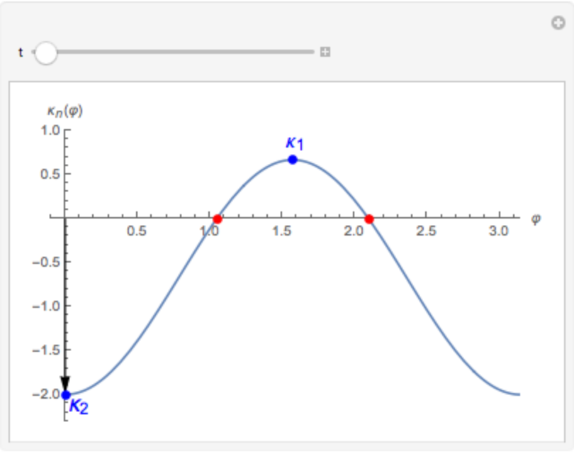
The normal curvature varying φ (principal curvatures have opposite signs in a hyperbolic point):

In[13]:=

$Manipulate[ Plot[-(2/3) (1 + 2 Cos[2 \[CurlyPhi]]), {\[CurlyPhi], 0, \[Pi]}, Epilog -> {Arrow[{{t, 0}, {t, -(2/3) (1 + 2 Cos[2 t])}}], Red, PointSize[.02], Point[{#, 0} & /@ zeroes], Blue, Point[{{0, -2}, {\[Pi]/2, 2/3}}], Text[Style["\!$\*SubscriptBox[\(\[Kappa]$, $2$]\)", 16], {.1, -2.1}], Text[Style["\!$\*SubscriptBox[ StyleBox[\"\[Kappa]\", \"TR\"], \(1$]\)", 16], {1.6, .9}]}, AxesLabel -> {\[CurlyPhi], "\!$\*SubscriptBox[\(\[Kappa]$, $n$]\)(\[CurlyPhi])"}, PlotRange -> {{-.1, \[Pi]}, {-2.3, 1}}], {t, 0, \[Pi]}]$

Out[13]=

The asymptotic directions correspond to the angles for the zeros:

In[14]:=

Out[14]=

In these directions, the normal curvature vanishes:

In[15]:=

Out[15]=

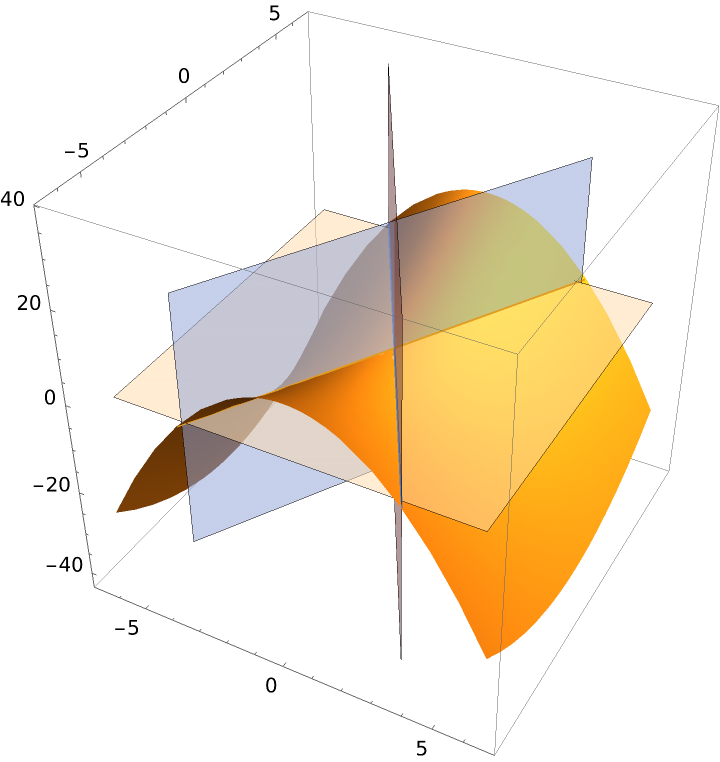
Plot the principal directions and the principal curves:

In[16]:=

$Show[ParametricPlot3D[{u, v, -u^2 + v^2/3}, {u, -2 \[Pi], 2 \[Pi]}, {v, -2 \[Pi], 2 \[Pi]}, BoxRatios -> {1, 1, 1}, Mesh -> None], Graphics3D[{Opacity[.5], Rotate[Polygon[ 4.5 {{\[Pi]/2, 0, -6}, {-\[Pi]/2, 0, -6}, {-\[Pi]/2, 0, 6}, {\[Pi]/2, 0, 6}}], \[Pi]/3, {0, 0, 1}], Rotate[Polygon[ 4.5 {{\[Pi]/2, 0, -8}, {-\[Pi]/2, 0, -8}, {-\[Pi]/2, 0, 8}, {\[Pi]/2, 0, 8}}], 2 \[Pi]/3, {0, 0, 1}], Polygon[{{6, -6, 0}, {-6, -6, 0}, {-6, 6, 0}, {6, 6, 0}}]}], ParametricPlot3D[{{-t, Sqrt[3] t, 0}, {t, Sqrt[3] t, 0}}, {t, -3.6, 3.6}]]$

Out[16]=

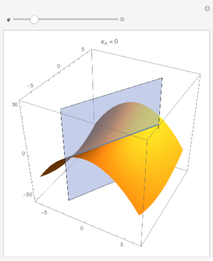
The normal sections and the normal curvature:

In[17]:=

$Manipulate[ Show[ParametricPlot3D[ hp, {u, -2 \[Pi], 2 \[Pi]}, {v, -2 \[Pi], 2 \[Pi]}, BoxRatios -> {1, 1, 1}, Mesh -> None, PlotLabel -> Row[{Subscript[\[Kappa], n], NumberForm[-(2/3) (1 + 2 Cos[2 \[CurlyPhi]]), {3, 2}]}, "="]], Graphics3D[{Opacity[.5], Rotate[Polygon[ 2 \[Pi] {{1, 0, -8}, {-1, 0, -8}, {-1, 0, 8}, {1, 0, 8}}], \[CurlyPhi], {0, 0, 1}]}], ParametricPlot3D[{u Cos[\[CurlyPhi]], v Sin[\[CurlyPhi]], -(u Cos[\[CurlyPhi]])^2 + (v Sin[\[CurlyPhi]])^2/3} /. {u -> t, v -> t}, {t, -2 \[Pi], 2 \[Pi]}]], {{\[CurlyPhi], \[Pi]/3}, 0., 2 \[Pi]}]$