Wolfram Function Repository
Instant-use add-on functions for the Wolfram Language
Function Repository Resource:
Perform Bayesian linear regression with conjugate priors
ResourceFunction["BayesianLinearRegression"][{{var11,var12,…,y1},{var21,var22,…,y2},…},{f1,f2,…},{var1,var2,…}] performs a Bayesian linear model fit on the data using basis functions fi with independent variables vari. | |
ResourceFunction["BayesianLinearRegression"][{{var11,var12,…}→y1,{var21,var22,…}→y2,…},…] generates the same result. | |
ResourceFunction["BayesianLinearRegression"][{{var11,var12,…},{var21,var22,…},…}→{y1,y2,…},…] generates the same result. |
| "PriorParameters" | values of the hyperparameters corresponding to the prior distribution of the fit coefficients. |
| "PosteriorParameters" | values of the hyperparameters corresponding to the posterior distribution of the fit coefficients. |
| "LogEvidence" | the natural log of the marginal likelihood |
| "Prior" | prior distributions. |
| "Posterior" | posterior distributions. |
| "Basis" | the basis functions supplied by the user. |
| "IndependentVariables" | the independent variables supplied by the user. |
| "Functions" | functions that yield distributions when applied arbitrary hyperparameters; only included when the "IncludeFunctions"→True option is set. |
| "PredictiveDistribution" | predictive distribution of the data. |
| "UnderlyingValueDistribution" | the distribution of of the fit line of the data. |
| "RegressionCoefficientDistribution" | marginal distribution of the fit coefficients. |
| "ErrorDistribution" | marginal distribution of the variance (for 1D regression) or covariance matrix. |
Generate a Bayesian linear regression on random data:
| In[1]:= |
| Out[1]= |  |
Generate test data:
| In[2]:= | ![data = RandomVariate[
MultinormalDistribution[( {
{1, 0.7},
{0.7, 1}
} )],
20
];
ListPlot[data]](https://www.wolframcloud.com/obj/resourcesystem/images/c66/c66f7392-efcc-42ca-949e-311fe403fb99/016164ebf0d34671.png) |
| Out[2]= | 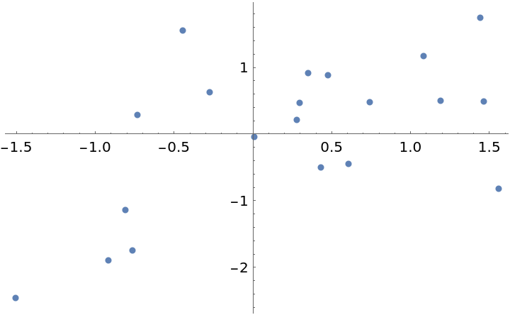 |
Fit the data with a first-order polynomial:
| In[3]:= |
| Out[3]= |
Show the predictive distribution of the model and the distribution of the fit line (dashed):
| In[4]:= | ![Show[
Plot[Evaluate@
InverseCDF[
linearModel["Posterior", "PredictiveDistribution"], {0.95, 0.5, 0.05}], {\[FormalX], -3, 3}, Filling -> {1 -> {2}, 3 -> {2}}, PlotLegends -> Table[Quantity[i, "Percent"], {i, {95, 50, 5}}]],
Plot[Evaluate@
InverseCDF[
linearModel["Posterior", "UnderlyingValueDistribution"], {0.95, 0.5, 0.05}], {\[FormalX], -3, 3}, Filling -> {1 -> {2}, 3 -> {2}}, PlotStyle -> Dashed],
ListPlot[data, PlotStyle -> Black],
PlotRange -> All
]](https://www.wolframcloud.com/obj/resourcesystem/images/c66/c66f7392-efcc-42ca-949e-311fe403fb99/5a73fe47f85494d0.png) |
| Out[4]= | 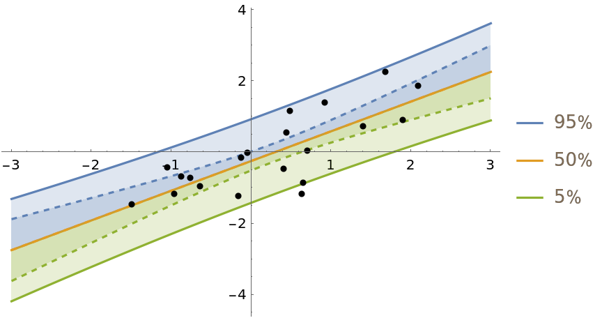 |
Plot the joint distribution of the coefficients a and b in the regression equation y=ax+b:
| In[5]:= | ![With[{
coefficientDist = linearModel["Posterior", "RegressionCoefficientDistribution"]
},
ContourPlot[
Evaluate[PDF[coefficientDist, {a, b}]],
{a, -1, 1},
{b, 0, 2},
PlotRange -> {0, All}, PlotPoints -> 20, FrameLabel -> {"a", "b"}, ImageSize -> 400,
PlotLabel -> "Posterior PDF of regression coefficients"
]
]](https://www.wolframcloud.com/obj/resourcesystem/images/c66/c66f7392-efcc-42ca-949e-311fe403fb99/325ce298ce1532ae.png) |
| Out[5]= | 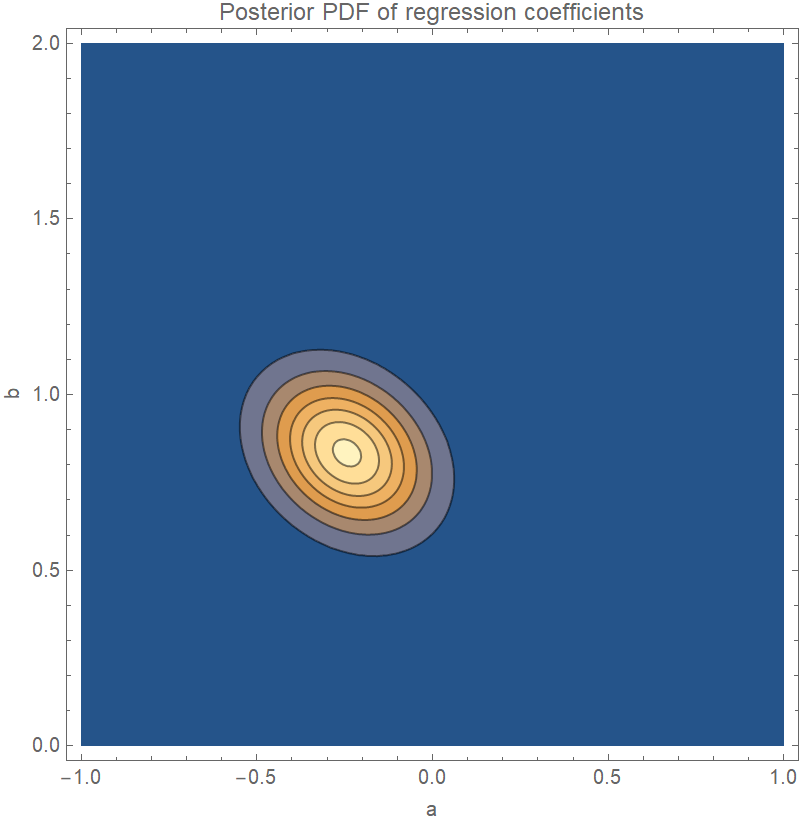 |
Plot the PDF of the posterior variance of the residuals:
| In[6]:= | ![With[{
errDist = linearModel["Posterior", "ErrorDistribution"]
},
Quiet@Plot[
Evaluate[PDF[errDist, e]],
{e, 0, 1},
PlotRange -> {0, All}, AxesLabel -> {"\!\(\*SuperscriptBox[\(\[Sigma]\), \(2\)]\)", "Density"}, ImageSize -> 400,
Filling -> Axis,
PlotLabel -> "Posterior PDF of residual variance"
]
]](https://www.wolframcloud.com/obj/resourcesystem/images/c66/c66f7392-efcc-42ca-949e-311fe403fb99/270e84b3f406a28b.png) |
| Out[6]= | 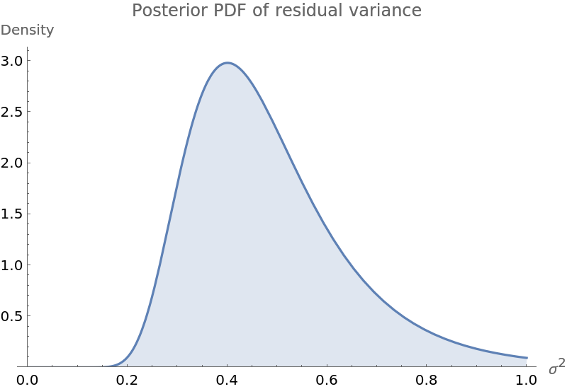 |
Fit the data with a polynomial of arbitrary degree and compare the prediction bands and log-evidence of fits up to degree 4:
| In[7]:= | ![Table[
Module[{
model = ResourceFunction["BayesianLinearRegression"][
Rule @@@ data, \[FormalX]^Range[0, degree], \[FormalX]],
predictiveDist
},
predictiveDist = model["Posterior", "PredictiveDistribution"];
Show[
Plot[Evaluate@
InverseCDF[predictiveDist, {0.95, 0.5, 0.05}], {\[FormalX], -3, 3}, Filling -> {1 -> {2}, 3 -> {2}}, PlotLegends -> Table[Quantity[i, "Percent"], {i, {95, 50, 5}}]],
ListPlot[data, PlotStyle -> Black],
PlotRange -> All,
PlotLabel -> StringForm["Degree: `1`\nLog evidence: `2`", degree, model["LogEvidence"] ]
]
],
{degree, 0, 4}
]](https://www.wolframcloud.com/obj/resourcesystem/images/c66/c66f7392-efcc-42ca-949e-311fe403fb99/761192f7aeeeb8ad.png) |
| Out[7]= | 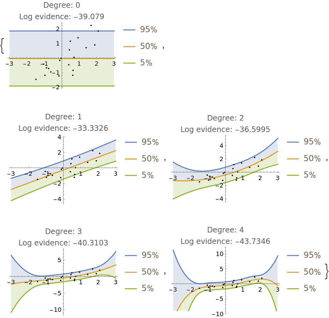 |
BayesianLinearRegression can do multivariate regression. For example, generate some 3D data:
| In[8]:= | ![data = RandomVariate[
MultinormalDistribution[{0, 0, 2}, RandomVariate[
InverseWishartMatrixDistribution[5, IdentityMatrix[3]]]],
50
];
ListPointPlot3D[data]](https://www.wolframcloud.com/obj/resourcesystem/images/c66/c66f7392-efcc-42ca-949e-311fe403fb99/207039f1a9b8f473.png) |
| Out[8]= | 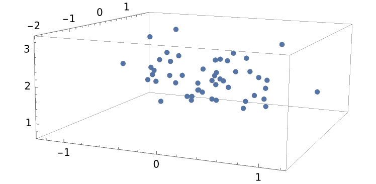 |
Do a regression where the x-coordinate is treated as the independent variable and y and z are both dependent on x:
| In[9]:= |
| Out[9]= |  |
The predictive joint distribution for y and z is a MultivariateTDistribution:
| In[10]:= |
| Out[10]= |  |
Visualize the joint distribution as an animation:
| In[11]:= | ![ListAnimate[
Table[
ContourPlot[
Evaluate[PDF[multiRegressionDist, {y, z}]],
{y, -3, 3},
{z, -3, 3},
PlotRange -> All,
FrameLabel -> {"y", "z"},
PlotLabel -> StringForm["x = `1`", \[FormalX]],
PlotPoints -> 20
],
{\[FormalX], -1.5, 1.5, 0.1}
],
AnimationRunning -> False
]](https://www.wolframcloud.com/obj/resourcesystem/images/c66/c66f7392-efcc-42ca-949e-311fe403fb99/01a08f6768f87389.png) |
| Out[11]= | 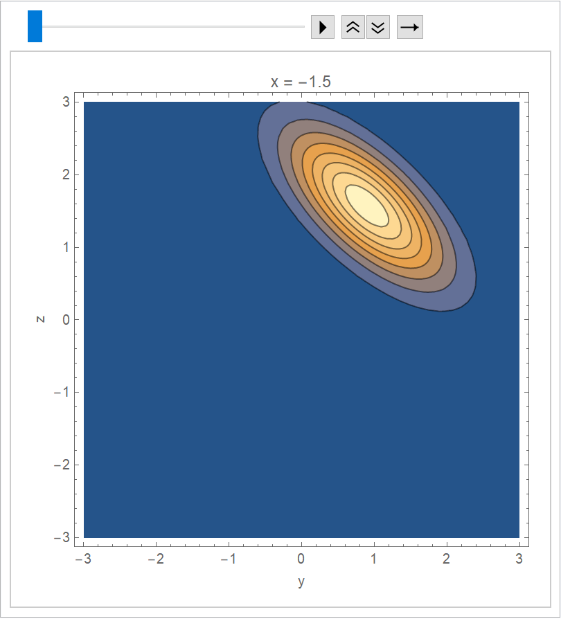 |
Just like LinearModelFit, BayesianLinearRegression constructs a model with bias term by default:
| In[12]:= | ![data = Range[-2, 2] -> Range[-2, 2] + 1 + RandomVariate[NormalDistribution[], 5];
model = ResourceFunction["BayesianLinearRegression"][
data, \[FormalX], \[FormalX]];
Show[
Plot[
Evaluate[
InverseCDF[
model["Posterior", "PredictiveDistribution"], {0.95, 0.5, 0.05}]],
{\[FormalX], -3, 3},
Filling -> {1 -> {2}, 3 -> {2}}
],
ListPlot[Transpose[List @@ data]]
]](https://www.wolframcloud.com/obj/resourcesystem/images/c66/c66f7392-efcc-42ca-949e-311fe403fb99/4b7ff1cb0f646f39.png) |
| Out[12]= | 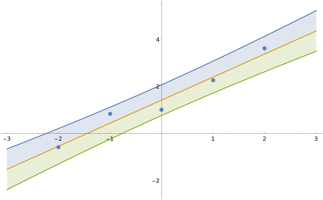 |
Force the intercept to be zero:
| In[13]:= | ![model2 = ResourceFunction["BayesianLinearRegression"][
data, \[FormalX], \[FormalX], IncludeConstantBasis -> False];
Show[
Plot[
Evaluate[
InverseCDF[
model2["Posterior", "PredictiveDistribution"], {0.95, 0.5, 0.05}]],
{\[FormalX], -3, 3},
Filling -> {1 -> {2}, 3 -> {2}}
],
ListPlot[Transpose[List @@ data]]
]](https://www.wolframcloud.com/obj/resourcesystem/images/c66/c66f7392-efcc-42ca-949e-311fe403fb99/7218cb068b47830a.png) |
| Out[13]= | 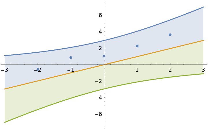 |
The prior can be specified in the same format as the parameter outputs of the Bayesian linear regression. This can be used to update a model with new observations. To illustrate this, generate some test data and divide the dataset into two parts:
| In[14]:= | ![data = TakeDrop[ SortBy[First]@RandomVariate[MultinormalDistribution[{0, 1}, ( {
{1, -1.3},
{-1.3, 2}
} )], 20], 10];
plot = ListPlot[data]](https://www.wolframcloud.com/obj/resourcesystem/images/c66/c66f7392-efcc-42ca-949e-311fe403fb99/2c1645f7fe636efd.png) |
| Out[14]= | 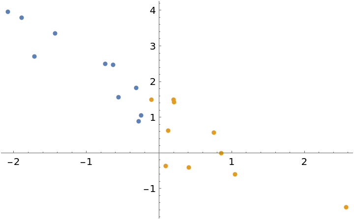 |
Fit the first half of the data:
| In[15]:= | ![model1 = ResourceFunction["BayesianLinearRegression"][
Rule @@@ data[[1]], \[FormalX], \[FormalX]];
Show[
Plot[Evaluate@InverseCDF[
model1["Posterior", "PredictiveDistribution"],
{0.95, 0.5, 0.05}
], {\[FormalX], -2, 2}, Filling -> {1 -> {2}, 3 -> {2}}],
plot
]](https://www.wolframcloud.com/obj/resourcesystem/images/c66/c66f7392-efcc-42ca-949e-311fe403fb99/389f4e144c3e1b9d.png) |
| Out[15]= | 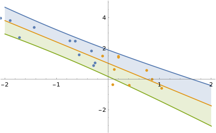 |
Use the posterior parameters of model1 as the prior to update the model with the second half of the dataset:
| In[16]:= | ![model2 = ResourceFunction["BayesianLinearRegression"][
Rule @@@ data[[2]], \[FormalX], \[FormalX], "PriorParameters" -> model1["PosteriorParameters"]];
Show[
Plot[Evaluate@InverseCDF[
model2["Posterior", "PredictiveDistribution"],
{0.95, 0.5, 0.05}
], {\[FormalX], -2, 2}, Filling -> {1 -> {2}, 3 -> {2}}],
plot
]](https://www.wolframcloud.com/obj/resourcesystem/images/c66/c66f7392-efcc-42ca-949e-311fe403fb99/0aa2b3d6145b2964.png) |
| Out[16]= | 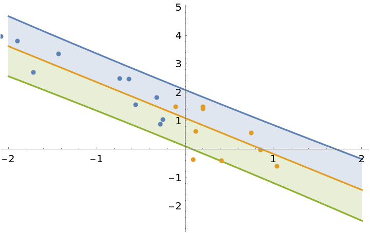 |
The result is exactly the same as when you would fit all of the data in a single step:
| In[17]:= | ![model3 = ResourceFunction["BayesianLinearRegression"][
Rule @@@ (Join @@ data), \[FormalX], \[FormalX]];
Column[{
model3["PosteriorParameters"],
model2["PosteriorParameters"]
}]](https://www.wolframcloud.com/obj/resourcesystem/images/c66/c66f7392-efcc-42ca-949e-311fe403fb99/38ff06b0dae9eb35.png) |
| Out[17]= |  |
When "IncludeFunctions"→True, the returned association contains the key "Functions". This key holds the functions that can be used to generate distributions from arbitrary values of hyperparameters:
| In[18]:= | ![data = Range[-2, 2] -> Range[-2, 2] + RandomVariate[NormalDistribution[], 5];
model = ResourceFunction["BayesianLinearRegression"][
data, \[FormalX], \[FormalX], "IncludeFunctions" -> True];
Keys@model["Functions"]](https://www.wolframcloud.com/obj/resourcesystem/images/c66/c66f7392-efcc-42ca-949e-311fe403fb99/369285418a9ea4cc.png) |
| Out[18]= |
The posterior distribution is obtained from the predictive distribution function:
| In[19]:= |
| Out[19]= |
Apply it to the posterior parameters:
| In[20]:= |
| Out[20]= |
Here is a dataset where it is unclear if the fit should be first or second order:
| In[21]:= |
| Out[21]= | 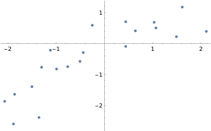 |
Fit the data with polynomials up to fourth degree, rank the log-evidences and inspect them:
| In[22]:= | ![models = AssociationMap[
ResourceFunction["BayesianLinearRegression"][
Rule @@@ data, \[FormalX]^Range[0, #], \[FormalX]] &,
Range[0, 4]
];
ReverseSort@models[[All, "LogEvidence"]]](https://www.wolframcloud.com/obj/resourcesystem/images/c66/c66f7392-efcc-42ca-949e-311fe403fb99/45ba2609062bcb9c.png) |
| Out[22]= |
Calculate the weights for each fit:
| In[23]:= | ![weights = Normalize[
(* subtract the max to reduce rounding error *)
Exp[models[[All, "LogEvidence"]] - Max[models[[All, "LogEvidence"]]]],
Total
];
ReverseSort[weights]](https://www.wolframcloud.com/obj/resourcesystem/images/c66/c66f7392-efcc-42ca-949e-311fe403fb99/2b22dbe61b9bbbbd.png) |
| Out[23]= |
Because the weights for the first and second order fits are so close, the correct Bayesian treatment is to include both in the final regression. Define a mixture of posterior predictive distributions:
| In[24]:= | ![mixDist = MixtureDistribution[
Values[weights],
Values@models[[All, "Posterior", "PredictiveDistribution"]]
];
Short /@ mixDist](https://www.wolframcloud.com/obj/resourcesystem/images/c66/c66f7392-efcc-42ca-949e-311fe403fb99/478035e1f8d15b19.png) |
| Out[24]= |  |
Compare the mixture fit to the individual polynomial regressions:
| In[25]:= | ![TabView[
KeyValueMap[
#1 -> Show[
Plot[
Evaluate@InverseCDF[#2, {0.95, 0.5, 0.05}],
{\[FormalX], -5, 5},
Filling -> {1 -> {2}, 3 -> {2}}, PlotLegends -> Table[Quantity[i, "Percent"], {i, {95, 50, 5}}],
PlotLabel -> Replace[
Lookup[weights, #1, None],
n_?NumericQ :> StringForm["Weight: `1`", n]
]
],
plot
] &,
Prepend[
models[[All, "Posterior", "PredictiveDistribution"]],
"Mixture" -> mixDist
]
]
]](https://www.wolframcloud.com/obj/resourcesystem/images/c66/c66f7392-efcc-42ca-949e-311fe403fb99/5c40921314363285.png) |
| Out[25]= | 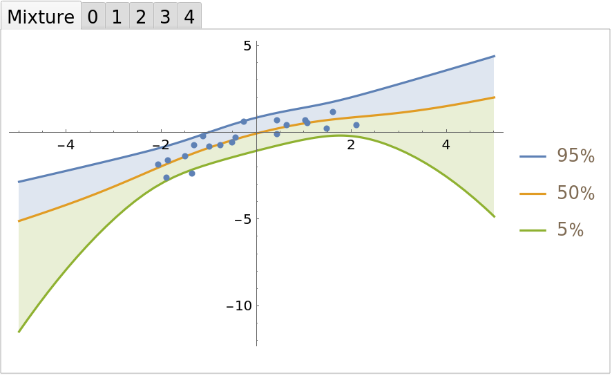 |
Symbolically calculate the predictive posterior after a single observation for any prior:
| In[26]:= | ![model = ResourceFunction[
"BayesianLinearRegression"][{xobs -> yobs}, \[FormalX], \[FormalX],
"PriorParameters" -> <|"B" -> {b1, b2}, "Lambda" -> {{l11^2, r l11 l22}, {r l11 l22, l22}}, "V" -> v, "Nu" -> nu|>];
dist[{xobs_, yobs_}, {b1_, b2_}, {l11_, l22_, r_}, v_, nu_] = Assuming[
v > 0 && nu > 0 && {xobs, yobs, \[FormalX], b1, b2, l11, l22} \[Element] Reals && -1 < r < 1,
FullSimplify[model["Posterior", "PredictiveDistribution"]]
]](https://www.wolframcloud.com/obj/resourcesystem/images/c66/c66f7392-efcc-42ca-949e-311fe403fb99/66c9d40827009890.png) |
| Out[26]= |  |
Visualize the prediction bands:
| In[27]:= | ![Manipulate[
Plot[
Evaluate@Thread@Tooltip[
InverseCDF[
dist[pt, b, {Sqrt[l11], Sqrt[l22], r}, v, nu], {0.95, 0.5, 0.05}],
Table[Quantity[i, "Percent"], {i, {95, 50, 5}}]
],
{\[FormalX], -10, 10},
PlotRange -> {-20, 20},
ImageSize -> Large,
Filling -> {1 -> {2}, 3 -> {2}}
],
{{pt, {0, 0}}, {-10, -10}, {10, 10}, ControlType -> Locator},
{{b, {0, 0}}, {-10, -10}, {10, 10}},
{{l11, 0.01}, 0.0001, 0.1},
{{l22, 0.01}, 0.0001, 0.1},
{{r, 0}, -1, 1},
{{v, 0.1}, 0.0001, 1},
{{nu, 0.1}, 0.0001, 1},
SaveDefinitions -> True
]](https://www.wolframcloud.com/obj/resourcesystem/images/c66/c66f7392-efcc-42ca-949e-311fe403fb99/66d8e6ad5778d3e3.png) |
| Out[27]= | 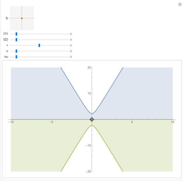 |
This work is licensed under a Creative Commons Attribution 4.0 International License