Function Repository Resource:

GeneralizedHelicoid

Compute the generalized helicoid of a curve

Contributed by: Wolfram Staff (original content by Alfred Gray)

ResourceFunction["GeneralizedHelicoid"][c,sl,v]

gives the generalized helicoid using slant sl and parameter v for the plane curve c.

Details and Options

Let α be a plane curve and write α(t)=(φ(t),ψ(t)). The generalized helicoid with profile curve α and slant sl is the surface parametrized by (cos(u)φ(v),sin(u)φ(v),sl(u)+ψ(v)).

The surface parameter v should not also be the parameter of the plane curve c.

Examples

Basic Examples (4)

Define a cissoid:

In[1]:=

$cissoid[a_][t_] := {(2 a t^2)/(1 + t^2), (2 a t^3)/(1 + t^2)}$

Plot it:

In[2]:=

Out[2]=

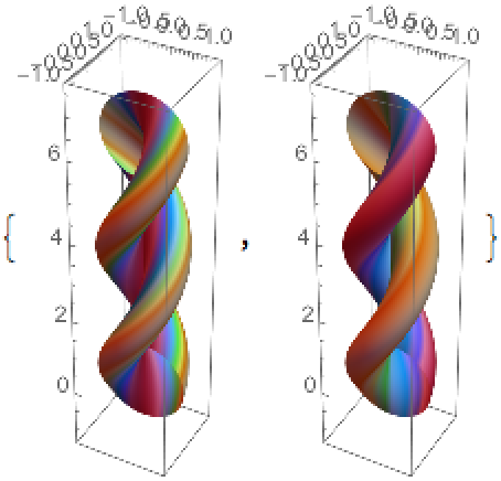
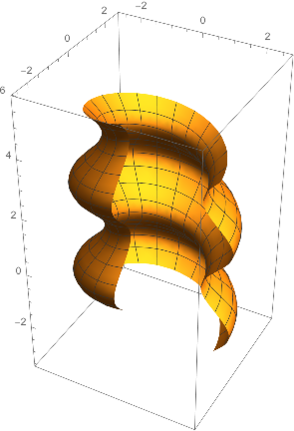
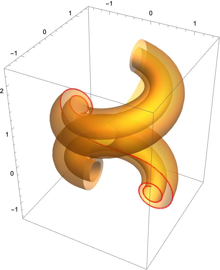
The generalized helicoid of a cissoid:

In[3]:=

Out[3]=

Plot the resulting surface:

In[4]:=

Out[4]=

Scope (2)

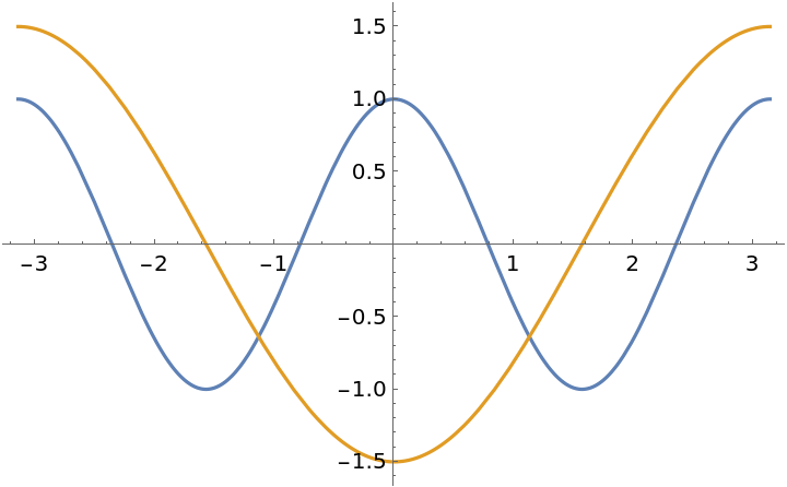
The generalized helicoid of a sinusoidal curve:

In[5]:=

Out[5]=

Plot the resulting surface:

In[6]:=

$ParametricPlot3D[Evaluate[singh], {u, 0, 3 Pi/2}, {v, -\[Pi], \[Pi]}]$

Out[6]=

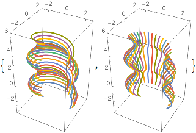
Plot parallel helical curves and meridians:

In[7]:=

${ParametricPlot3D[ Evaluate[Table[singh, {v, -\[Pi], \[Pi], \[Pi]/12}]], {u, 0, 3 \[Pi]/2}], ParametricPlot3D[ Evaluate[ Table[singh, {u, 0, 3 \[Pi]/2, \[Pi]/16}]], {v, -\[Pi], \[Pi]}]}$

Out[7]=

A surface is a flat generalized helicoid if its profile curve can be parametrized as α(t)=(t,ψ(t)), where :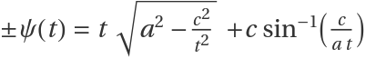

In[8]:=

$zcprofile[pm_, a_, c_][t_] := {t, pm (t Sqrt[a^2 - c^2/t^2] + c ArcSin[c/(a t)])}$

A flat generalized helicoid (for simplicity we set a=c=1):

In[9]:=

Out[9]=

Being flat means having zero Gaussian curvature. The Gaussian curvature of a surface can be computed via the resource function GaussianCurvature:

In[10]:=

Out[143]=

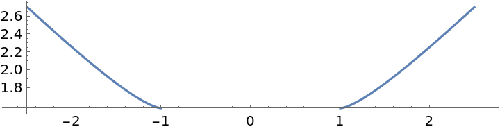
Plot the zero-curvature profile curves:

In[144]:=

Out[144]=

Plot the flat generalized helicoid for these curves:

In[145]:=

$Show[ParametricPlot3D[ ResourceFunction["GeneralizedHelicoid"][zcprofile[#, 1, 1][v], 2, u] & /@ {-1, 1} // Evaluate, {u, 0, 9 \[Pi]/2}, {v, 1, 5}, PlotPoints -> {40, 10}]]$

Out[145]=

Properties and Relations (2)

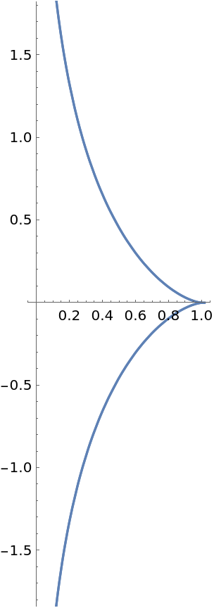
Define a tractrix:

In[146]:=

$tractrix[a_, b_][t_] := {a Sin[t], b (Cos[t] + Log[Tan[t/2]])}$

Plot it:

In[147]:=

$ParametricPlot[tractrix[1, 1][v], {v, 0, 4 \[Pi]}]$

Out[147]=

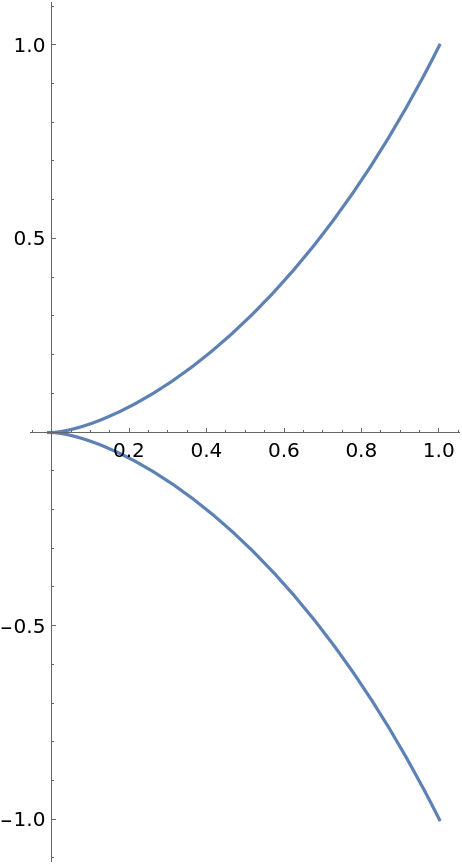
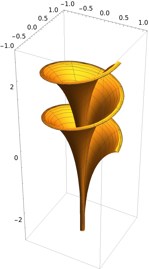
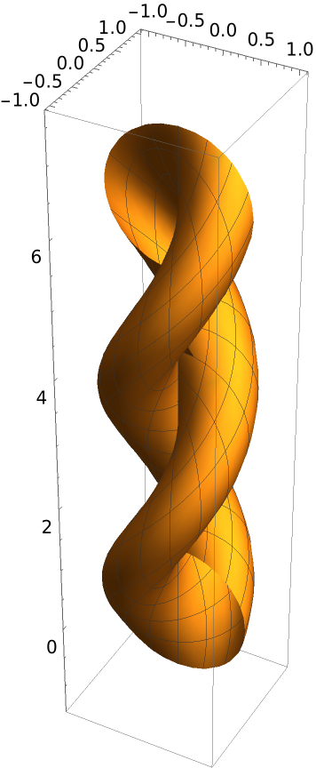
Compute the generalized helicoid of a tractrix:

In[148]:=

Out[148]=

Plot the generalized helicoid:

In[149]:=

Out[149]=

The generalized helicoid of a tractrix is a surface of Dini:

In[150]:=

Out[150]=

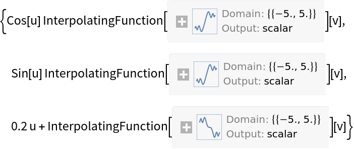
Here is some code to create a curve with prescribed (intrinsic) curvature:

In[151]:=

$intrinsic[f_, a_, {c_, d_, e_}, {min_, max_}][t_] := Module[{x, y, \[Theta], s}, eqic = {x'[s] == Cos[\[Theta][s]], y'[s] == Sin[\[Theta][s]], \[Theta]'[s] == f[s], x[a] == c, y[a] == d, \[Theta][a] == e}; sol = NDSolve[eqic, {x, y, \[Theta]}, {s, min, max}]; {x[t], y[t]} /. sol[[1]] ]$

Define a curve with linear intrinsic curvature:

In[152]:=

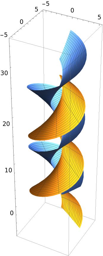
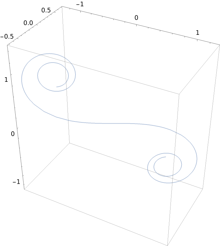
The generalized helicoid for the previous curvature:

In[153]:=

Out[153]=

Plot the profile curve:

In[154]:=

Out[154]=

Plot the generalized helicoid surface for a linear intrinsic curvature (profile curve in red):

In[155]:=

$Show[ParametricPlot3D[ Evaluate[ ResourceFunction["GeneralizedHelicoid"][f[v], 0.2, u]], {u, 0, 3 \[Pi]/2}, {v, -5, 5}, PlotPoints -> {30, 60}, Mesh -> False, PlotStyle -> Opacity[.5], MaxRecursion -> 3], ParametricPlot3D[ Evaluate[ResourceFunction["GeneralizedHelicoid"][f[v], 0.2, u]] /. u -> 0, {v, -5, 5}, Mesh -> False, PlotStyle -> {Opacity[.5], Red}, MaxRecursion -> 3]]$

Out[155]=

Properties and Relations (7)

A generalized helix of a circle:

In[156]:=

Out[156]=

A twisphere has a parametrization of a generalized helix type:

In[157]:=

$twisphere[a_, b_][u_, v_] := {a Cos[u] Cos[v], a Sin[u] Cos[v], a Sin[v] + b u}$

In[158]:=

Plot the twisphere:

In[159]:=

$ParametricPlot3D[Evaluate[ts], {u, 0, 2 \[Pi]}, {v, -\[Pi], \[Pi]}]$

Out[159]=

Compute the Gaussian curvature with the resource function GaussianCurvature:

In[160]:=

Out[161]=

Compute mean curvature with the resource function MeanCurvature:

In[162]:=

Out[162]=

Plot both curvatures:

In[163]:=

$Plot[{Cos[2 v], -((3 Cos[v])/2)}, {v, -\[Pi], \[Pi]}]$

Out[163]=

Plot the twisphere according to both curvatures:

In[164]:=

$ParametricPlot3D[ Evaluate[twisphere[1, 1][u, v]], {u, 0, 2 \[Pi]}, {v, -\[Pi], \[Pi]}, Lighting -> True, PlotPoints -> {40, 40}, Mesh -> False, MeshFunctions -> Function[{x, y, z, u, v}, #], ColorFunction -> Function[{x, y, z, u, v}, ColorData["BrightBands"][#]], ColorFunctionScaling -> False, ImageSize -> Small] & /@ {Rescale[ gcur, {-1, 1}], Rescale[mcur, {-1.5, 1.5}]}$

Out[164]=

Publisher

Enrique Zeleny

Version History

1.0.0 – 27 April 2020

Source Metadata

Citation:
- Abbena, E., Salamon, S., Gray, A., Modern Differential Geometry of Curves and Surfaces with Mathematica, 3rd ed. Boca Raton, FL: Chapman & Hall/CRC, 2006.

License Information

This work is licensed under a Creative Commons Attribution 4.0 International License