Wolfram Function Repository
Instant-use add-on functions for the Wolfram Language
Function Repository Resource:
Fast numerical estimation of the power spectral density or the cross spectral density
ResourceFunction["WelchSpectralEstimate"][data,rate] estimates the data power spectral density at a given rate. | |
ResourceFunction["WelchSpectralEstimate"][data1,data2,rate] estimates the data cross spectral density at a given rate. |
| "SegmentSize" | Automatic | the number of datapoints to use in a Fourier transform |
| "OverlapOffset" | Automatic | the offset between segments to average or a fraction of the possible offset (defaults to half of the "SegmentSize") |
| FourierParameters | {0,1} | Fourier convention parameters |
| "Window" | Automatic | the spectral window to apply to the data (if appropriate, the HannWindow will be chosen) |
| "OneSided" | True | True to evaluate only the first half of the Fourier transform, otherwise False for evaluating the whole range |
| "Reduction" | Mean | the function to average the segments together |
| "DensityScaling" | True | True for scaling as a density, False for spectrogram scaling |
| "Detrend" | "Constant" | the level of detrending to apply to the data segments, before transformation |
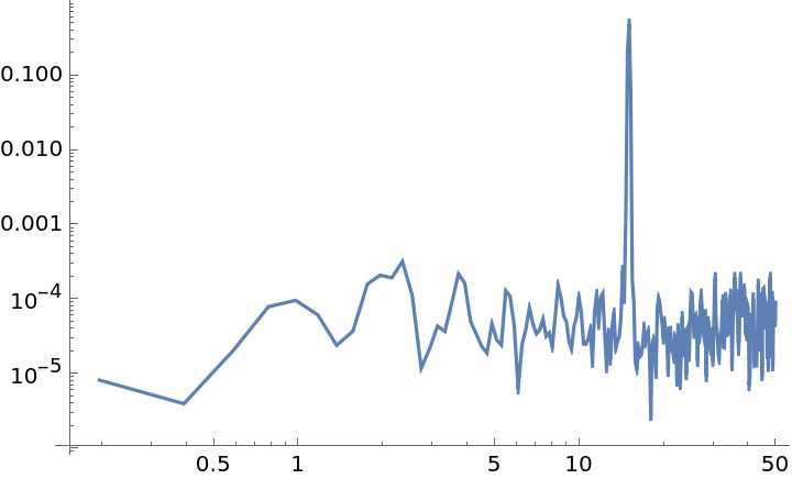
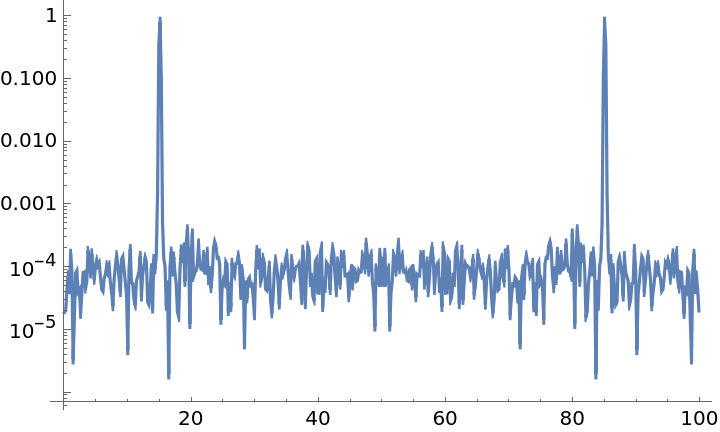
Calculate the spectral density of a random data sample:
| In[1]:= | ![data = Sin[15*2 Pi*Range[0, 10, 0.01]] + RandomVariate[NormalDistribution[0, 0.1], 1001];
ListLogLogPlot[
ResourceFunction[
"WelchSpectralEstimate", ResourceSystemBase -> "https://www.wolframcloud.com/obj/resourcesystem/api/1.0"][data, 100.0], Joined -> True]](https://www.wolframcloud.com/obj/resourcesystem/images/bbe/bbee4715-d7fe-426a-a646-e433c01a904d/2d450928f4f5bdf8.png) |
| Out[2]= | 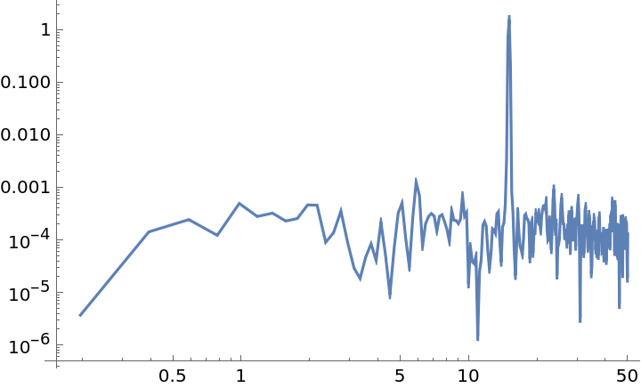 |
Evaluate the Cross Spectral Density (CSD) of two sinusoidal, noisy datasets and display amplitude and phase:
| In[3]:= | ![data1 = Sin[15*2 Pi*Range[0, 10, 0.01]] + RandomVariate[NormalDistribution[0, 0.1], 1001];
data2 = 0.3 Sin[15*2 Pi*Range[0, 10, 0.01] + 0.5] + Sin[10*2 Pi*Range[0, 10, 0.01]] + RandomVariate[NormalDistribution[0, 0.1], 1001];
csd = ResourceFunction[
"WelchSpectralEstimate", ResourceSystemBase -> "https://www.wolframcloud.com/obj/resourcesystem/api/1.0"][data1, data2, 100.0];
{ListLogLogPlot[Abs[csd], Joined -> True], ListLogLinearPlot[{#1, Arg@#2} & @@@ csd, Joined -> True]}](https://www.wolframcloud.com/obj/resourcesystem/images/bbe/bbee4715-d7fe-426a-a646-e433c01a904d/3439a4016f58f5cb.png) |
| Out[6]= |  |
Compare the influence of different spectral windows on the PSD:
| In[7]:= | ![data = Sin[15*2 Pi*Range[0, 10, 0.01]] + RandomVariate[NormalDistribution[0, 0.001], 1001];
windows = {DirichletWindow, HannWindow, HammingWindow, BlackmanHarrisWindow, KaiserWindow};
ListLogLogPlot[
ResourceFunction[
"WelchSpectralEstimate", ResourceSystemBase -> "https://www.wolframcloud.com/obj/resourcesystem/api/1.0"][data, 100.0, "Window" -> #] & /@ windows, Joined -> True, PlotLegends -> windows]](https://www.wolframcloud.com/obj/resourcesystem/images/bbe/bbee4715-d7fe-426a-a646-e433c01a904d/0c46b21d8c769e26.png) |
| Out[9]= | 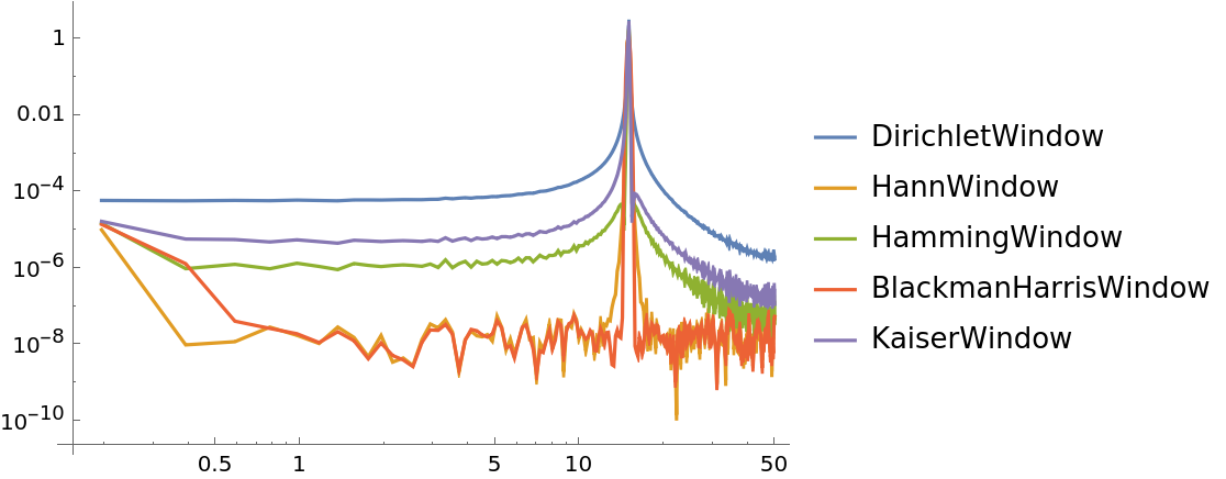 |
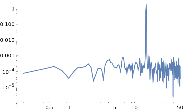
"SegmentSize" sets number of data points from which to calculate the Fourier transform; smaller numbers means more averaging but lower resolution:
| In[10]:= | ![data = Sin[15*2 Pi*Range[0, 10, 0.001]] + RandomVariate[NormalDistribution[0, 0.1], 10001];
ListLogLogPlot[
ResourceFunction[
"WelchSpectralEstimate", ResourceSystemBase -> "https://www.wolframcloud.com/obj/resourcesystem/api/1.0"][data, 100.0, "SegmentSize" -> #], Joined -> True, PlotLabel -> #] & /@ {200, 500, 1000, 5000, 10000}](https://www.wolframcloud.com/obj/resourcesystem/images/bbe/bbee4715-d7fe-426a-a646-e433c01a904d/18e80f89f2c2cefe.png) |
| Out[11]= | 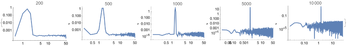 |
"OverlapOffset" allows to set the distance of the starting point between two partitioned segments; a smaller integer number means closer overlaps and thus more averaging:
| In[12]:= | ![data = Sin[15*2 Pi*Range[0, 10, 0.01]] + RandomVariate[NormalDistribution[0, 0.1], 1001];
ListLogLogPlot[
ResourceFunction[
"WelchSpectralEstimate", ResourceSystemBase -> "https://www.wolframcloud.com/obj/resourcesystem/api/1.0"][data, 100.0, "OverlapOffset" -> #], Joined -> True, PlotLabel -> #] & /@ {1, 511}](https://www.wolframcloud.com/obj/resourcesystem/images/bbe/bbee4715-d7fe-426a-a646-e433c01a904d/5d30891cc228b957.png) |
| Out[13]= | 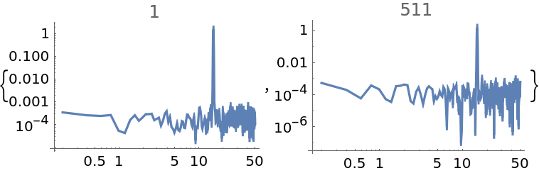 |
"OverlapOffset" also allows the specification of an overlap fraction of the number of data points minus the segment size, as a real number between zero and one:
| In[14]:= | ![data = Sin[15*2 Pi*Range[0, 10, 0.01]] + RandomVariate[NormalDistribution[0, 0.1], 1001];
ListLogLogPlot[
ResourceFunction[
"WelchSpectralEstimate", ResourceSystemBase -> "https://www.wolframcloud.com/obj/resourcesystem/api/1.0"][data, 100.0, "OverlapOffset" -> #], Joined -> True, PlotLabel -> #] & /@ {0.01, 0.99}](https://www.wolframcloud.com/obj/resourcesystem/images/bbe/bbee4715-d7fe-426a-a646-e433c01a904d/6a2dfba084db7741.png) |
| Out[15]= | 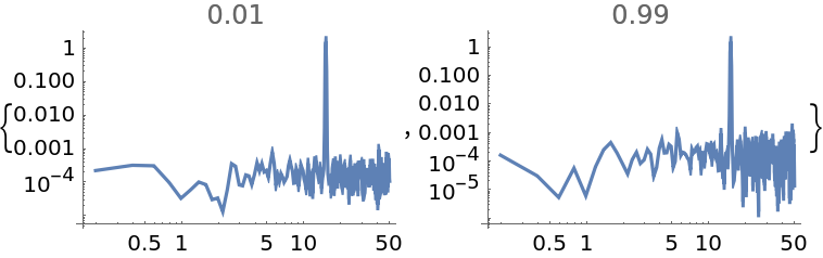 |
Sets the FourierParameters option for the respective Fourier transforms:
| In[16]:= | ![data = Sin[15*2 Pi*Range[0, 10, 0.01]] + RandomVariate[NormalDistribution[0, 0.1], 1001];
ListLogLogPlot[
ResourceFunction[
"WelchSpectralEstimate", ResourceSystemBase -> "https://www.wolframcloud.com/obj/resourcesystem/api/1.0"][data, 100.0, FourierParameters -> {1, -1}], Joined -> True]](https://www.wolframcloud.com/obj/resourcesystem/images/bbe/bbee4715-d7fe-426a-a646-e433c01a904d/5ac03f73e17abaa2.png) |
| Out[17]= | 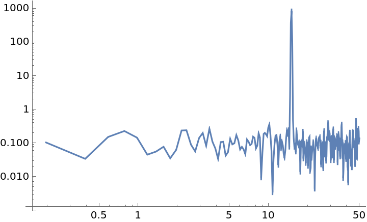 |
Use the "Window" option to specify windowing functions:
| In[18]:= | ![data = Sin[15*2 Pi*Range[0, 10, 0.001]] + RandomVariate[NormalDistribution[0, 0.1], 10001];
ListLogLogPlot[{
ResourceFunction[
"WelchSpectralEstimate", ResourceSystemBase -> "https://www.wolframcloud.com/obj/resourcesystem/api/1.0"][data, 100.0, "Window" -> DirichletWindow],
ResourceFunction[
"WelchSpectralEstimate", ResourceSystemBase -> "https://www.wolframcloud.com/obj/resourcesystem/api/1.0"][data, 100.0, "Window" -> HannWindow]
}, Joined -> True, PlotLegends -> {"Dirichlet", "Hann"}]](https://www.wolframcloud.com/obj/resourcesystem/images/bbe/bbee4715-d7fe-426a-a646-e433c01a904d/23e97da324e5d056.png) |
| Out[19]= | 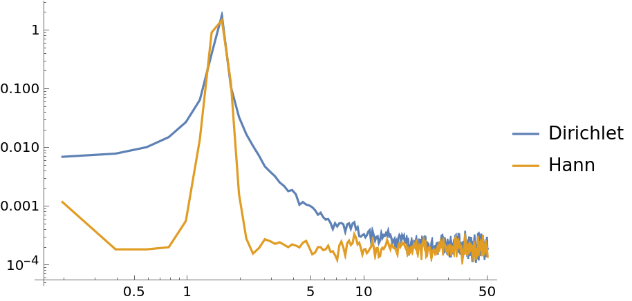 |
A list can be applied as the window function, provided the length is equal to its segment size:
| In[20]:= | ![data = Sin[15*2 Pi*Range[0, 10, 0.001]] + RandomVariate[NormalDistribution[0, 0.1], 10001];
segmentSize = 1024;
windowPoints = PDF[NormalDistribution[0, 0.1], Subdivide[-1, 1, segmentSize - 1]];
ListLogLogPlot[{ResourceFunction[
"WelchSpectralEstimate", ResourceSystemBase -> "https://www.wolframcloud.com/obj/resourcesystem/api/1.0"][data, 100.0, "SegmentSize" -> segmentSize, "Window" -> windowPoints]}, Joined -> True]](https://www.wolframcloud.com/obj/resourcesystem/images/bbe/bbee4715-d7fe-426a-a646-e433c01a904d/7638fd9014f42266.png) |
| Out[23]= | 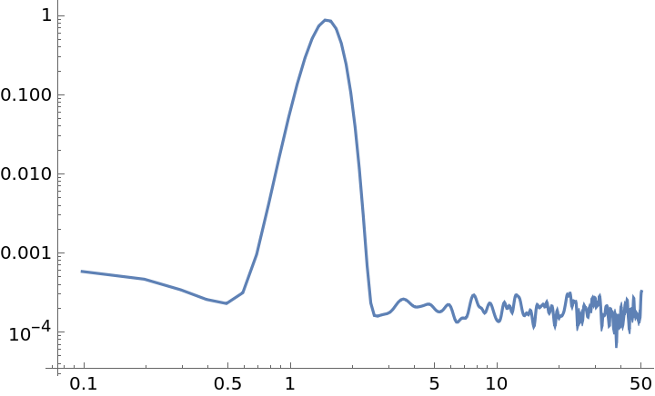 |
Set a custom function as the window:
| In[24]:= | ![data = Sin[15*2 Pi*Range[0, 10, 0.001]] + RandomVariate[NormalDistribution[0, 0.1], 10001];
ListLogLogPlot[{
ResourceFunction[
"WelchSpectralEstimate", ResourceSystemBase -> "https://www.wolframcloud.com/obj/resourcesystem/api/1.0"][data, 100.0, "Window" -> (Exp[-50 #^2] &)],
ResourceFunction[
"WelchSpectralEstimate", ResourceSystemBase -> "https://www.wolframcloud.com/obj/resourcesystem/api/1.0"][data, 100.0, "Window" -> (HannWindow[#, 0.4] &)]
}, Joined -> True]](https://www.wolframcloud.com/obj/resourcesystem/images/bbe/bbee4715-d7fe-426a-a646-e433c01a904d/05f026a86cc85d46.png) |
| Out[25]= | 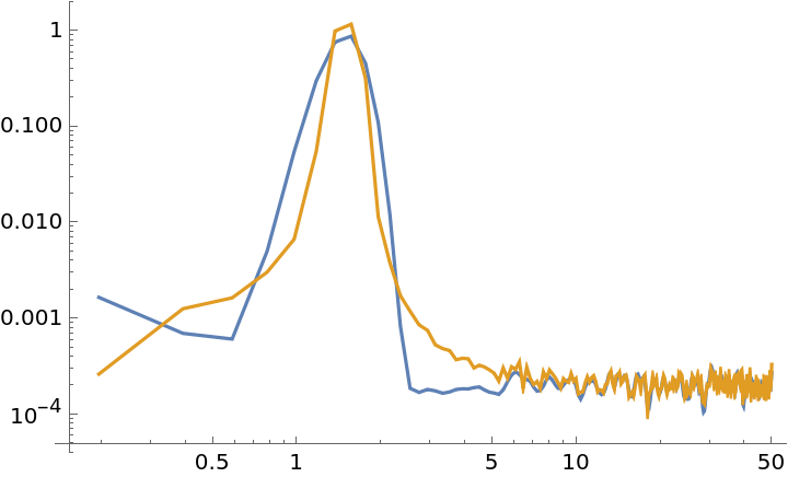 |
The "Detrend" option can be used to detrend the initial data segments before transformations occur. The option can be specified with string arguments for constant or linear detrends:
| In[32]:= | ![(* Evaluate this cell to get the example input *) CloudGet["https://www.wolframcloud.com/obj/46c45b74-61b5-4a63-800d-c72ae9151993"]](https://www.wolframcloud.com/obj/resourcesystem/images/bbe/bbee4715-d7fe-426a-a646-e433c01a904d/637784ad79d897f3.png) |
| Out[33]= | 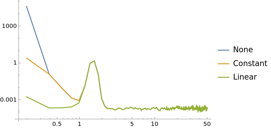 |
A list of integers can be specified instead which polynomial orders should be detrended:
| In[34]:= | ![data = Sin[15*2 Pi*Range[0, 10, 0.001]] + 10*Range[0, 10, 0.001] + 10*Range[0, 10, 0.001]^2 + 10*Range[0, 10, 0.001]^3 + 100 + RandomVariate[NormalDistribution[0, 0.1], 10001];
ListLogLogPlot[{
ResourceFunction[
"WelchSpectralEstimate", ResourceSystemBase -> "https://www.wolframcloud.com/obj/resourcesystem/api/1.0"][data, 100.0, "Detrend" -> None],
ResourceFunction[
"WelchSpectralEstimate", ResourceSystemBase -> "https://www.wolframcloud.com/obj/resourcesystem/api/1.0"][data, 100.0, "Detrend" -> {0, 1, 2, 3}]
}, Joined -> True, PlotLegends -> {"None", "Detrend: \!\(\*SuperscriptBox[\(x\), \(3\)]\), \!\(\*SuperscriptBox[\(x\), \(2\)]\), x, \!\(\*SuperscriptBox[\(x\), \(0\)]\)"}]](https://www.wolframcloud.com/obj/resourcesystem/images/bbe/bbee4715-d7fe-426a-a646-e433c01a904d/15df134bb32a4cc2.png) |
| Out[35]= | 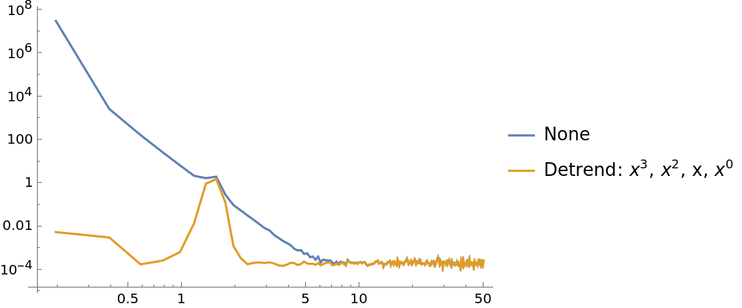 |
Investigate the frequency response on white noise data for different kind of filters:
| In[36]:= | ![(* Evaluate this cell to get the example input *) CloudGet["https://www.wolframcloud.com/obj/2fcbd4d5-dc4b-4f70-b5ab-5f681dc9ddd7"]](https://www.wolframcloud.com/obj/resourcesystem/images/bbe/bbee4715-d7fe-426a-a646-e433c01a904d/71742083624abcb2.png) |
| Out[40]= | 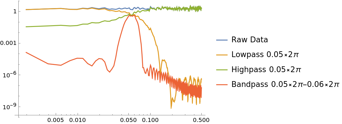 |
Estimate the system transfer function of a set state and its measured response:
| In[41]:= | ![time = Range[0, 10, 0.05];
data = Table[Round[Mod[x, 1]] - 0.5, {x, time}];
dataResponse = NDSolveValue[{u'[
t] == (Interpolation[Transpose[{time, data}], InterpolationOrder -> 0][t] - u[t]), u[0] == 0}, u, {t, Min[time], Max[time]}] /@ time;
csd = ResourceFunction[
"WelchSpectralEstimate", ResourceSystemBase -> "https://www.wolframcloud.com/obj/resourcesystem/api/1.0"][data, dataResponse, 0.05, "Window" -> KaiserWindow];
psd = ResourceFunction[
"WelchSpectralEstimate", ResourceSystemBase -> "https://www.wolframcloud.com/obj/resourcesystem/api/1.0"][data, 0.05, "Window" -> KaiserWindow];
transferFunction = Transpose[{csd[[All, 1]], csd[[All, 2]]/psd[[All, 2]]}];
phase = Arg[transferFunction[[All, 2]]];
{
ListLogLogPlot[{#1, Abs@#2} & @@@ transferFunction, Joined -> True, PlotLabel -> "Abs of frequency response", ImageSize -> Medium],
ListLogLinearPlot[{#1, 180/Pi*Arg@#2} & @@@ transferFunction, Joined -> True, PlotRange -> All, PlotLabel -> "Phase of frequency response", ImageSize -> Medium]
}](https://www.wolframcloud.com/obj/resourcesystem/images/bbe/bbee4715-d7fe-426a-a646-e433c01a904d/1f62f1599ff3d14d.png) |
| Out[48]= | 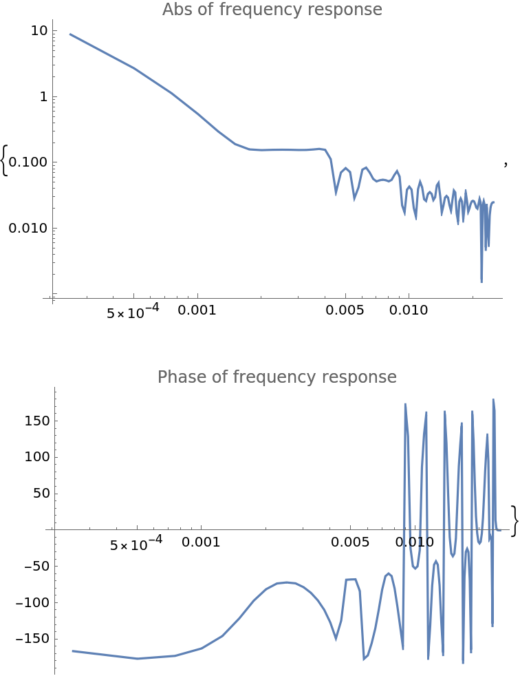 |
Even for complex input, the "OneSided" option will still remain True by default and thus return only the front of the Fourier transform:
| In[49]:= |
| Out[49]= |
Estimate the uncertainty of the Fourier deviations by just choosing a different reduction function:
| In[50]:= | ![data = Sin[15*2 Pi*Range[0, 10, 0.01]] + RandomVariate[NormalDistribution[0, 0.001], 1001];
ListLogLogPlot[
ResourceFunction[
"WelchSpectralEstimate", ResourceSystemBase -> "https://www.wolframcloud.com/obj/resourcesystem/api/1.0"][data, 100.0, "Reduction" -> MeanAround]]](https://www.wolframcloud.com/obj/resourcesystem/images/bbe/bbee4715-d7fe-426a-a646-e433c01a904d/08a754884bf82391.png) |
| Out[51]= | 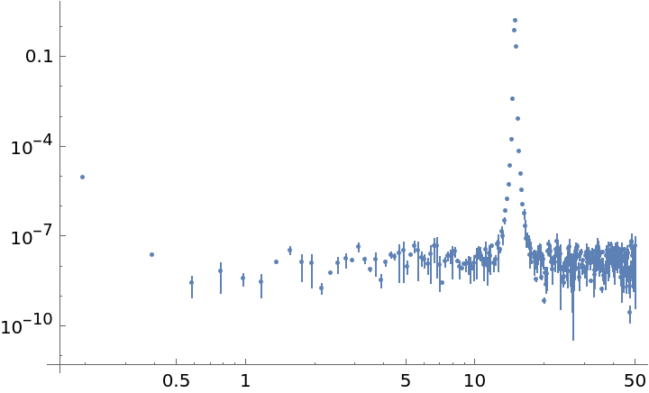 |
This work is licensed under a Creative Commons Attribution 4.0 International License
![data = Sin[15*2 Pi*Range[0, 10, 0.01]] + RandomVariate[NormalDistribution[0, 0.1], 1001];
ListLogPlot[{ResourceFunction[
"WelchSpectralEstimate", ResourceSystemBase -> "https://www.wolframcloud.com/obj/resourcesystem/api/1.0"][data, 100.0, "OneSided" -> False]}, Joined -> True, PlotRange -> All]](https://www.wolframcloud.com/obj/resourcesystem/images/bbe/bbee4715-d7fe-426a-a646-e433c01a904d/54b09fa1f978e970.png)
![data = Sin[15*2 Pi*Range[0, 10, 0.01]] + RandomVariate[NormalDistribution[0, 0.1], 1001];
ListLogLogPlot[{ResourceFunction[
"WelchSpectralEstimate", ResourceSystemBase -> "https://www.wolframcloud.com/obj/resourcesystem/api/1.0"][data, 100.0, "Reduction" -> Median]}, Joined -> True]](https://www.wolframcloud.com/obj/resourcesystem/images/bbe/bbee4715-d7fe-426a-a646-e433c01a904d/0721af6030345ebd.png)
![data = Sin[15*2 Pi*Range[0, 10, 0.01]] + RandomVariate[NormalDistribution[0, 0.1], 1001];
ListLogLogPlot[{ResourceFunction[
"WelchSpectralEstimate", ResourceSystemBase -> "https://www.wolframcloud.com/obj/resourcesystem/api/1.0"][data, 100.0, "DensityScaling" -> False]}, Joined -> True, PlotRange -> All]](https://www.wolframcloud.com/obj/resourcesystem/images/bbe/bbee4715-d7fe-426a-a646-e433c01a904d/4a84e8cd2d8753c5.png)