Wolfram Function Repository
Instant-use add-on functions for the Wolfram Language
Function Repository Resource:
Construct an interpolating polynomial approximation of a function using the Padua points
ResourceFunction["PaduaInterpolation"][expr,{x,xmin,xmax},{y,ymin,ymax}] evaluates expr with x running from xmin to xmax and y running from ymin to ymax, and constructs a ResourceFunction["PaduaInterpolation"] object which represents an approximate bivariate function corresponding to the result. | |
ResourceFunction["PaduaInterpolation"][…][x,y] evaluates the interpolating function with particular arguments x and y. |
| InterpolationOrder | 15 | order of the interpolating polynomial generated |
| "PaduaType" | 1 | type of Padua points to use |
| WorkingPrecision | MachinePrecision | the precision used in internal computations |
Construct the Padua interpolant corresponding to the function Sin[π x+Sin[π y]]:
| In[1]:= |
See the value at zero:
| In[2]:= |
| Out[2]= |
Plot the Padua interpolant along with the original function:
| In[3]:= |
| Out[3]= | 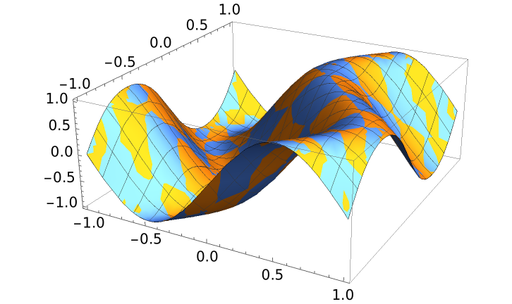 |
See an interpolation function:
| In[4]:= |
| Out[4]= |
Get values for a few points:
| In[5]:= |
| Out[5]= |
A test function due to Franke:
| In[6]:= | ![franke[x_, y_] := 3/4 Exp[-(((9 x - 2)^2 + (9 y - 2)^2)/4)] + 3/4 Exp[-((9 x + 1)^2/49) - (9 y + 1)/10] + 1/2 Exp[-(((9 x - 7)^2 + (9 y - 3)^2)/4)] - 1/5 Exp[-(9 x - 4)^2 - (9 y - 7)^2]](https://www.wolframcloud.com/obj/resourcesystem/images/ba0/ba0a5841-af57-4613-8868-63d03a273a39/33051e3231a6bcc9.png) |
Interpolate and plot over a rectangular domain:
| In[7]:= |
| Out[8]= | 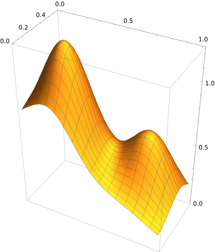 |
Construct a Padua interpolant of the Dixon–Szegö function of degree 25:
| In[9]:= | ![f = ResourceFunction[
"PaduaInterpolation"][(4 - 2.1 x^2 + x^4/3) x^2 + x y + 4 (y^2 - 1) y^2, {x, -2, 2}, {y, -1.25, 1.25}, InterpolationOrder -> 25];
ContourPlot[f[x, y], {x, -2, 2}, {y, -1.25, 1.25}, AspectRatio -> Automatic, Contours -> 20]](https://www.wolframcloud.com/obj/resourcesystem/images/ba0/ba0a5841-af57-4613-8868-63d03a273a39/38829b2da6d3a933.png) |
| Out[9]= |  |
Use type 3 Padua points in interpolating the Dixon–Szegö function:
| In[10]:= | ![f = ResourceFunction[
"PaduaInterpolation"][(4 - 2.1 x^2 + x^4/3) x^2 + x y + 4 (y^2 - 1) y^2, {x, -2, 2}, {y, -1.25, 1.25}, "PaduaType" -> 3];
ContourPlot[f[x, y], {x, -2, 2}, {y, -1.25, 1.25}, AspectRatio -> Automatic, Contours -> 20]](https://www.wolframcloud.com/obj/resourcesystem/images/ba0/ba0a5841-af57-4613-8868-63d03a273a39/5835e7528313d99d.png) |
| Out[10]= | 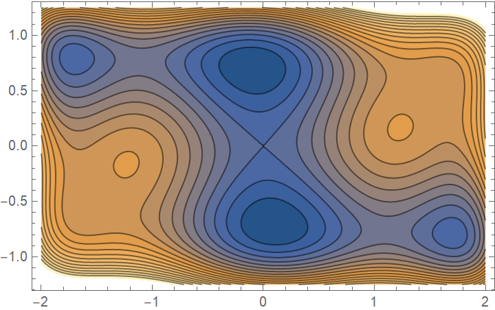 |
Use 25-digit precision in the interpolation:
| In[11]:= | ![f = ResourceFunction[
"PaduaInterpolation"][(4 - 21/10 x^2 + x^4/3) x^2 + x y + 4 (y^2 - 1) y^2, {x, -2, 2}, {y, -(5/4), 5/4}, WorkingPrecision -> 25];
f[1, 1]](https://www.wolframcloud.com/obj/resourcesystem/images/ba0/ba0a5841-af57-4613-8868-63d03a273a39/3241241ecf94ac3e.png) |
| Out[11]= |
If the input function is a polynomial of degree k, PaduaInterpolation reproduces the original polynomial as long as k is less than the setting for InterpolationOrder:
| In[12]:= |
| Out[13]= | 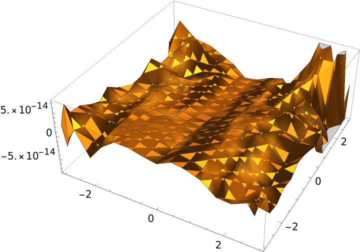 |
A test function due to Franke:
| In[14]:= | ![franke[x_, y_] := 3/4 Exp[-(((9 x - 2)^2 + (9 y - 2)^2)/4)] + 3/4 Exp[-((9 x + 1)^2/49) - (9 y + 1)/10] + 1/2 Exp[-(((9 x - 7)^2 + (9 y - 3)^2)/4)] - 1/5 Exp[-(9 x - 4)^2 - (9 y - 7)^2]](https://www.wolframcloud.com/obj/resourcesystem/images/ba0/ba0a5841-af57-4613-8868-63d03a273a39/51f37d294d28bccb.png) |
Use the resource function PaduaPoints with InterpolatingPolynomial to construct a Padua interpolant:
| In[15]:= |
| Out[15]= |  |
Use PaduaInterpolation to construct a Padua interpolant:
| In[16]:= |
The interpolant constructed using InterpolatingPolynomial evaluates faster, but the interpolant generated by PaduaInterpolation gives a more accurate answer:
| In[17]:= |
| Out[17]= |
| In[18]:= |
| Out[18]= |
This work is licensed under a Creative Commons Attribution 4.0 International License