Wolfram Function Repository
Instant-use add-on functions for the Wolfram Language
Function Repository Resource:
Compute the binormal surface to a curve
ResourceFunction["BinormalSurface"][c,t,{u,v}] computes the binormal surface of a curve c with parameter t using u and v to parametrize the result. |
Define and plot a helix curve:
| In[1]:= |
| Out[1]= |
| In[2]:= |
| Out[2]= | 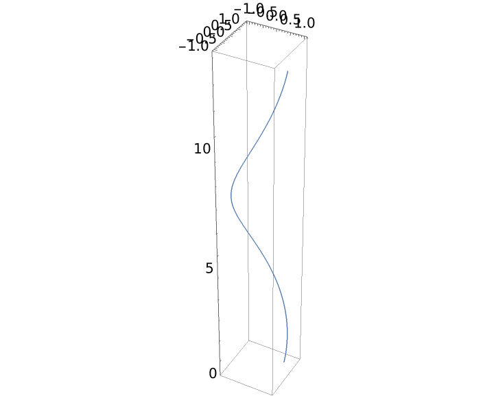 |
Compute the normal surface of the helix curve with the resource function NormalSurface and plot the result:
| In[3]:= |
| Out[3]= |
| In[4]:= |
| Out[4]= | 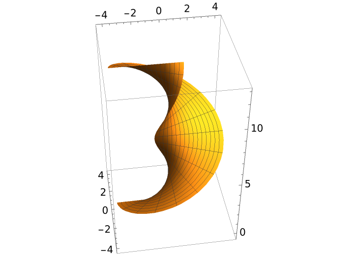 |
Compute and plot the binormal surface of the helix curve:
| In[5]:= |
| Out[5]= |
| In[6]:= | ![bsp = ParametricPlot3D[
Evaluate[ResourceFunction["BinormalSurface"][helix, t, {u, v}]], {u,
0, 2 \[Pi]}, {v, 0, 5}, PlotPoints -> {20, 10}]](https://www.wolframcloud.com/obj/resourcesystem/images/b6a/b6a1f628-e71e-4a42-9ae0-9497f46a6f3e/732124682de253d5.png) |
| Out[6]= | 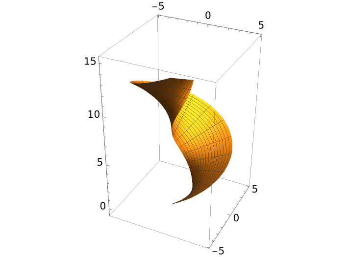 |
Show both surfaces along with the helix curve:
| In[7]:= |
| Out[7]= | 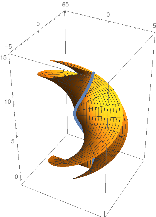 |
This work is licensed under a Creative Commons Attribution 4.0 International License