Function Repository Resource:

KernelSimilarity

Source Notebook

Calculate the pairwise similarity between vectors or matrices using kernel functions

Contributed by: Felipe Amorim

ResourceFunction["KernelSimilarity"][x]

calculates the pairwise kernel similarities of x with itself.

ResourceFunction["KernelSimilarity"][x,y]

calculates the pairwise kernel similarity between x and y.

Details and Options

Kernels (or kernel functions) are measurements of similarity between pairs of vectors or matrices. They are used heavily in various machine learning algorithms called kernel methods to compute pairwise similarities between a set of training data points and itself.

If x and y are vectors, ResourceFunction["KernelSimilarity"] returns a single value k(x,y), where k is the kernel function. If x and y are matrices, ResourceFunction["KernelSimilarity"] returns the kernel matrix (also known as the Gram matrix) with entries K_ij=k(x_i ,y_j).

ResourceFunction["KernelSimilarity"][x] is equivalent to ResourceFunction["KernelSimilarity"][x ,x].

The following option is supported:

"KernelType"

"RadialBasisFunction"

specifies the kernel function used to compute similarities

The "KernelType" option specifies which kernel function to use among the following options:

"Linear"

x.y +c

"Polynomial"

(γ(x.y) + c)^d

"Sigmoid"

Tanh[(γ(x.y)+c)]

"RadialBasisFunction"

Exp[-γ |x,y|²]

"Laplacian"

Exp[-γ |x,y|₁]

The following suboptions are supported:

"GammaValue"

1/n

the parameter γ in the kernels functions, where n is the dimension of the input vectors

"BiasParameter"

bias term c in polynomial and sigmoid kernels

"PolynomialDegree"

the degree of the polynomial d in the polynomial kernel

Not all suboptions are supported by every kernel type: "BiasParameter" is used only by "Linear", "Polynomial", and "Sigmoid"; "PolynomialDegree" only by "Polynomial"; and "GammaValue" by all kernels except "Linear". Suboptions irrelevant to the specified kernel result in failures.

Examples

Basic Examples (3)

Calculate the kernel similarity between two vectors:

In[1]:=

Out[1]=

Calculate the kernel similarity between two matrices:

In[2]:=

$ResourceFunction["KernelSimilarity"][\!$\* TagBox[ RowBox[{"(", "", GridBox[{ {"2", "3"}, {"3", "5"} }, GridBoxAlignment->{"Columns" -> {{Center}}, "Rows" -> {{Baseline}}}, GridBoxSpacings->{"Columns" -> { Offset[0.27999999999999997`], { Offset[0.7]}, Offset[0.27999999999999997`]}, "Rows" -> { Offset[0.2], { Offset[0.4]}, Offset[0.2]}}], "", ")"}], Function[BoxForm`e$, MatrixForm[BoxForm`e$]]]$, \!$\* TagBox[ RowBox[{"(", "", GridBox[{ {"1", "3"}, {"2", "7"} }, GridBoxAlignment->{"Columns" -> {{Center}}, "Rows" -> {{Baseline}}}, GridBoxSpacings->{"Columns" -> { Offset[0.27999999999999997`], { Offset[0.7]}, Offset[0.27999999999999997`]}, "Rows" -> { Offset[0.2], { Offset[0.4]}, Offset[0.2]}}], "", ")"}], Function[BoxForm`e$, MatrixForm[BoxForm`e$]]]$]$

Out[2]=

Calculate the kernel self-similarity of a matrix:

In[3]:=

Out[3]=

Options (4)

Use the "KernelType" option to modify the kernel function:

In[4]:=

Out[4]=

Use the "BiasParameter" option to modify the bias value used in the kernel function:

In[5]:=

Out[5]=

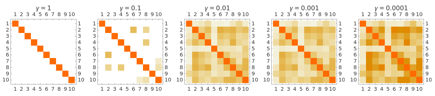
Use the "GammaValue" option to specify the gamma parameter used in the kernel function:

In[6]:=

Out[6]=

Lower gamma values make the kernel less sensitive to distance, producing similarity scores closer to 1:

In[7]:=

$m = RandomReal[{1, 100}, {10, 10}]; gammaValues = {1, 0.1, 0.01, 0.001, 0.0001}; GraphicsRow[ MatrixPlot[ ResourceFunction["KernelSimilarity"][m, "KernelType" -> {"RadialBasisFunction", "GammaValue" -> #}], PlotLabel -> \[Gamma] == #] & /@ gammaValues] // Quiet$

Out[8]=

Use the "PolynomialDegree" option to specify the degree of the polynomial kernel:

In[9]:=

Out[9]=

Compare it with the default value (d=3):

In[10]:=

Out[10]=

Applications (3)

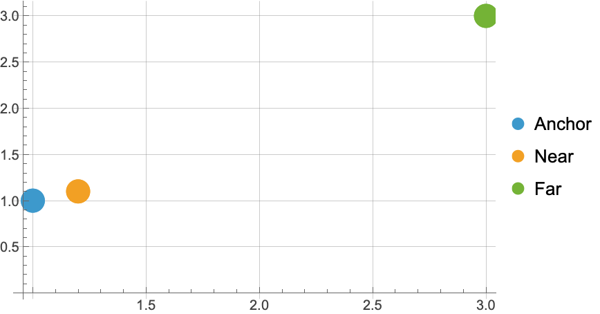
Define and visualize three points:

In[11]:=

anchor = {1, 1};
near = {1.2, 1.1};
far = {3, 3};
points = {anchor, near, far};
ListPlot[{{anchor}, {near}, {far}}, PlotStyle -> PointSize[0.05], PlotLegends -> {"Anchor", "Near", "Far"}, GridLines -> Automatic]

Out[12]=

Compute similarities between the anchor and the other points using different kernels:

In[13]:=

kernels = {"Linear", "Polynomial", "RadialBasisFunction", "Laplacian"};
similarities = Table[{k, ResourceFunction["KernelSimilarity"][anchor, near, "KernelType" -> k], ResourceFunction["KernelSimilarity"][anchor, far, "KernelType" -> k] // N}, {k, kernels}];

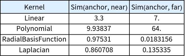
Display the results:

In[14]:=

Out[14]=

RBF (radial basis function) and Laplacian kernels measure similarity based on distance, assigning higher similarity to nearby points. On the other hand, linear and polynomial kernels depend on dot products, which capture alignment and magnitude rather than pure spatial proximity. This distinction is particularly important in machine learning applications, since distance-based kernels are well-suited for capturing local structure of the input data.

Properties and Relations (5)

In the case of matrices, KernelSimilarity calculates the similarity between every pair of vectors (known as the Gram Matrix):

In[15]:=

m1 = {{1, 2}, {3, 4}};
m2 = {{5, 6}, {7, 8}};
ResourceFunction["KernelSimilarity"][m1, m2] == Outer[ResourceFunction["KernelSimilarity"], m1, m2, 1]

Out[16]=

The self-similarity of a vector with the "RadialBasisFunction" kernel is always 1:

In[17]:=

Out[17]=

In the case of two normalized vectors, the linear kernel with bias equals zero returns the cosine similarity, meaning that 1- KernelSimilarity[v_1,v₂]=CosineDistance[v_1,v₂]:

In[18]:=

v1 = Normalize[{1, 2, 2}];
v2 = Normalize[{3, 9, 7}];
ResourceFunction["KernelSimilarity"][v1, v2, "KernelType" -> {"Linear", "BiasParameter" -> 0}]

Out[19]=

In[20]:=

Out[20]=

KernelSimilarity[a,b] is the same as :

In[21]:=

m1 = {{1, 2}, {4, 5}};
m2 = {{5, 1}, {8, 4}};
ResourceFunction["KernelSimilarity"][m1, m2] == Transpose[ResourceFunction["KernelSimilarity"][m2, m1]]

Out[22]=

The "RadialBasisFunction", "Laplacian" and "Polynomial" kernels always produce symmetric and positive semidefinite (PSD) Gram matrices:

In[23]:=

Out[24]=

However, the Sigmoid and Linear kernels may produce non-positive-semidefinite Gram matrices, which can cause issues when used in kernel methods that require PSD matrices:

In[25]:=