Basic Examples (2) 

Define a function of two variables taking as input a vector of variables:

In[1]:=

Out[1]=

Apply the function:

In[2]:=

Out[2]=

Scope (2) 

Use ScalarPureFunction to obtain a linear pure function of three variables and evaluate it at (1,-2,1):

In[3]:=

Out[3]=

In[4]:=

Out[4]=

Use ScalarPureFunction to obtain a transcendental pure function of three variables and evaluate it at (1,1,1):

In[5]:=

Out[5]=

In[6]:=

Out[6]=

Options (1) 

IndexingMethod (1) 

The IndexingMethod option allows specifying the method used to indexing elements of argvars in the ScalarPureFunction. By default, the method is set to "UseIndexed", which uses the Indexed function. Alternatively, can be set the option to "UsePart" to use the Part function. This option provides flexibility in choosing the preferred method of indexing elements of argvars within the ScalarPureFunction:

In[7]:=

Out[7]=

Applications (3) 

Generate a Height Map (1) 

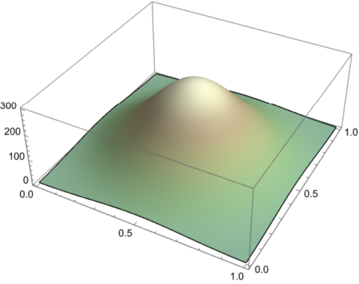
To generate a height map for an imaginary mountain in the shape of a two-dimensional Gaussian function, use ScalarPureFunction to represent the height at each point of the mountain as follows:

In[8]:=

Out[8]=

In[9]:=

Out[9]=

In[10]:=

Out[10]=

Poincaré Sections of Hamiltonian Systems with Two Degrees of Freedom (2) 

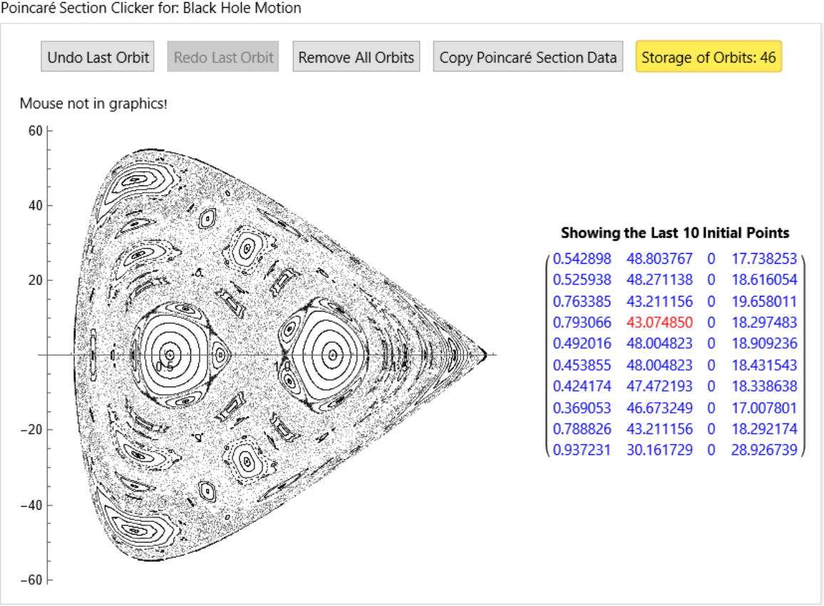
Use ScalarPureFunction in combination with ClickPoincarePlot2D to plot Poincaré sections of particle motion near a black hole horizon:

In[11]:=

In[12]:=

Out[12]=

Poincaré sections of the Yang-Mills-Higgs system:

In[13]:=

In[14]:=

Out[14]=

Properties and Relations (2) 

The function ScalarPureFunction shares some similarities with ResourceFunction["ExpressionToFunction"], which also converts expressions into pure functions. However, the two functions differ in their design and in how they handle the same use cases. Below is a comparison:

In[15]:=

Out[15]=

In[16]:=

Out[16]=

Use ScalarPureFunction in combination with ResourceFunction["TensorPureFunction"] to compute a Hessian matrix:

In[17]:=

Out[17]=

In[18]:=

Out[18]=

Possible Issues (3) 

If any of the specified variables have existing definitions, ScalarPureFunction issues a warning and returns unevaluated. For example:

In[19]:=

Out[21]=

To avoid this issue, wrap the variables with Block to prevent conflicts with global definitions:

In[22]:=

Out[22]=

Since ScalarPureFunction explicitly checks for global definitions before proceeding, it remains unevaluated when global definitions of the arguments are found. For example:

In[23]:=

In[24]:=

Out[24]=

Evaluate overrides the hold attribute so that ScalarPureFunction behaves as expected with the previously defined inputs:

In[25]:=

Out[25]=

On the other hand, when using Evaluate explicitly on the function or variable arguments before passing them to ScalarPureFunction, and at least one of the variables in the argument list has a global definition, the expected behavior of holding evaluation and issuing a warning will not occur. Instead, the function will be evaluated with the assigned values, potentially leading to incorrect results. For example:

In[26]:=

In[27]:=

Out[27]=

In this case, since Evaluate forces the immediate evaluation of the input, ScalarPureFunction does not detect existing global definitions and proceeds incorrectly. To avoid this issue, it is recommended to use Clear to remove any prior definitions before applying the function.