Wolfram Function Repository
Instant-use add-on functions for the Wolfram Language
Function Repository Resource:
Plot and find the area of a region determined by a list of points, the x axis and the type of boundary
ResourceFunction["DiscreteIntegralPlot"][data,method] plots the region determined by data, the x-axis and the type of boundary and prints the area of that the region. |
Plot data and determine the area of the region determined by data and the x-axis, using the left–hand endpoints as the height of the rectangles:
| In[1]:= | ![data = {{0, 0.8121}, {1, 1.3904}, {2, 2.8374}, {3, 3.1539}, {4, 4.134}, {5, 5.3356}, {6, 6.7651}, {7, 7.6077}, {8., 8.9556}, {9, 9.3877}, {10, 10.8627}, {11, 11.8943}, {12, 12.8101}, {13, 13.6069}, {14, 14.4239}, {15, 15.1200}, {16, 16.3355},
{17, 17.0501}, {18, 18.7869}, {19, 19.2568}, {20, 20.5573}, {21, 21.0866}, {22, 22.7888}, {23, 23.3589}, {24, 24.7452}, {25, 25.6962}, {26, 26.9515}, {27, 27.2051}, {28, 28.6112}, {29, 29.3606}, {30, 30.1864}, {31, 31.5974}, {32, 32.6556}, {33, 33.9730}, {34, 34.3237}, {35, 35.4104}, {36, 36.8455}, {37, 37.3661}, {38, 38.8999}, {39, 39.2904}, {40, 40.5100}};
ResourceFunction["DiscreteIntegralPlot"][data, Left]](https://www.wolframcloud.com/obj/resourcesystem/images/a99/a999c6cb-64c6-4191-b1ec-8a024d62a2de/3bd999b65b950233.png) |
| Out[2]= | 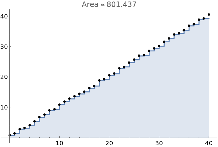 |
Use data given by a formula:
| In[3]:= |
| Out[4]= | 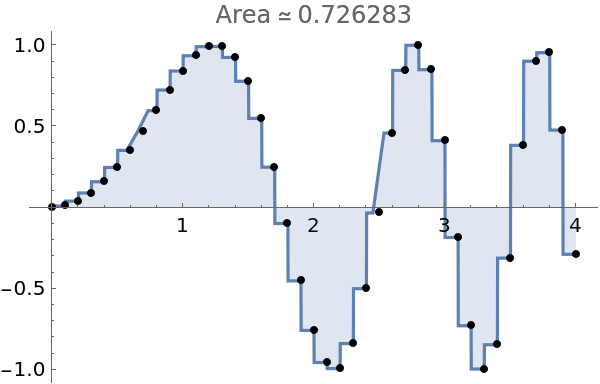 |
Note the bad spots in this graph around x=0.6 and x=2.5. Plotting more points fixes the problem:
| In[5]:= |
| Out[6]= | 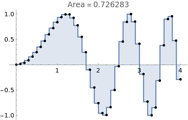 |
Apply a style to the region:
| In[7]:= |
| Out[8]= | 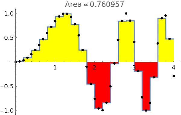 |
Apply a style to the points:
| In[9]:= | ![data1 = Table[{x, Sin[x^2]}, {x, 0, 4, .1}];
ResourceFunction["DiscreteIntegralPlot"][data1, Simpson, FillingStyle -> {Red, Yellow}, "PointStyle" -> {{PointSize[.02], Blue}}, ImageSize -> 300]](https://www.wolframcloud.com/obj/resourcesystem/images/a99/a999c6cb-64c6-4191-b1ec-8a024d62a2de/664a04e4d312b299.png) |
| Out[10]= | 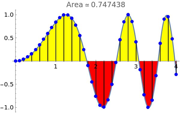 |
Use Manipulate to illustrate all possible methods to be used:
| In[11]:= | ![data1 = Table[{x, Sin[x^2]}, {x, 0, 4, .1}];
Manipulate[
ResourceFunction["DiscreteIntegralPlot"][data1, method, PlotPoints -> 60, FillingStyle -> {Red, Yellow}, ImageSize -> 300], {method, {Left, Midpoint, Right, Upper, Lower, Trap, Simpson, Spline}}]](https://www.wolframcloud.com/obj/resourcesystem/images/a99/a999c6cb-64c6-4191-b1ec-8a024d62a2de/556a07598320fecd.png) |
| Out[12]= | 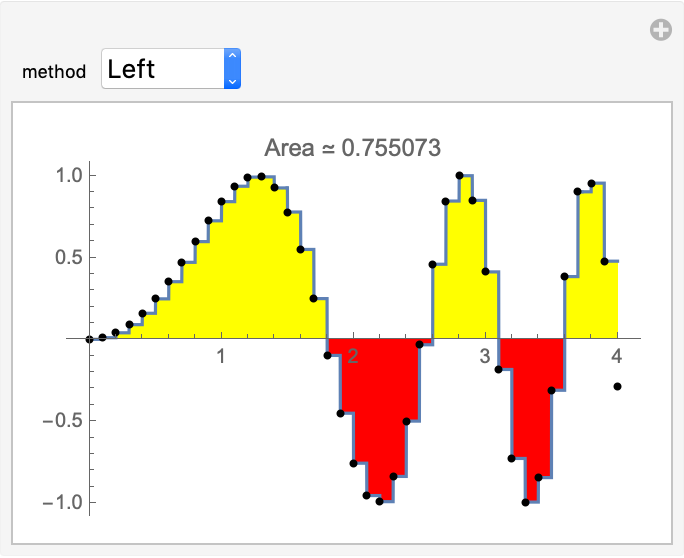 |
Setting the option "DrawGraph" to False suppresses the plot of the region and returns the area:
| In[13]:= |
| Out[14]= |
Data must be ordered:
| In[15]:= |
Simpson's method requires an even number of subintervals and the range should be chosen accordingly:
| In[16]:= | ![data1 = Table[{x, Sin[x^2]}, {x, 0, 4.1, .1}];
ResourceFunction["DiscreteIntegralPlot"][data1, Simpson, PlotPoints -> 60, FillingStyle -> {Red, Yellow}, ImageSize -> 300]](https://www.wolframcloud.com/obj/resourcesystem/images/a99/a999c6cb-64c6-4191-b1ec-8a024d62a2de/398aacab8c06d611.png) |
| In[17]:= |
| Out[17]= |
This work is licensed under a Creative Commons Attribution 4.0 International License