Wolfram Function Repository
Instant-use add-on functions for the Wolfram Language
Function Repository Resource:
Compute the unit normal of a surface
ResourceFunction["UnitNormal"][s,{u,v}] gives the unit normal vector field to the surface s parametrized by variables u,v. |
Define a torus surface:
| In[1]:= |
| Out[1]= |
Get the unit normals of the surface:
| In[2]:= |
| Out[2]= |
Plot the vector field:
| In[3]:= | ![Show[ParametricPlot3D[torus, {u, 0, \[Pi]}, {v, -\[Pi], \[Pi]}, PlotStyle -> Opacity[.5]], Graphics3D[{Arrowheads[0.02], Arrow /@ Table[{torus, torus + normals}, {u, 0, \[Pi], 2 \[Pi]/20}, {v, -\[Pi], \[Pi], 2 \[Pi]/20}]}]]](https://www.wolframcloud.com/obj/resourcesystem/images/9f3/9f36e694-e56f-4026-b221-f6e9ec01bbe1/1340146fc8165619.png) |
| Out[3]= | 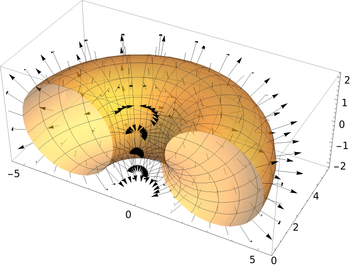 |
Define a Möbius strip:
| In[4]:= |
| Out[4]= |
Get the unit normals of the surface:
| In[5]:= |
| Out[5]= |  |
A Gauss map is not well defined on the whole surface, as unit normal vectors are only defined up to sign and there is no way to consistently decide the direction of the normal vector:
| In[6]:= | ![Show[ParametricPlot3D[mobius, {u, 0, 2}, {v, 0, 4 \[Pi]}, PlotPoints -> 40], Graphics3D[{Arrowheads[0.02], Arrow /@ Table[{mobius, mobius + normals}, {u, 0, 2, .5}, {v, -2 \[Pi], 2 \[Pi], 2 \[Pi]/20}]}]]](https://www.wolframcloud.com/obj/resourcesystem/images/9f3/9f36e694-e56f-4026-b221-f6e9ec01bbe1/445ce3b9586b0e9e.png) |
| Out[6]= | 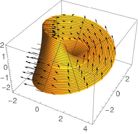 |
Define a sine surface:
| In[7]:= |
| Out[7]= |
Plot the sine surface:
| In[8]:= |
| Out[8]= | 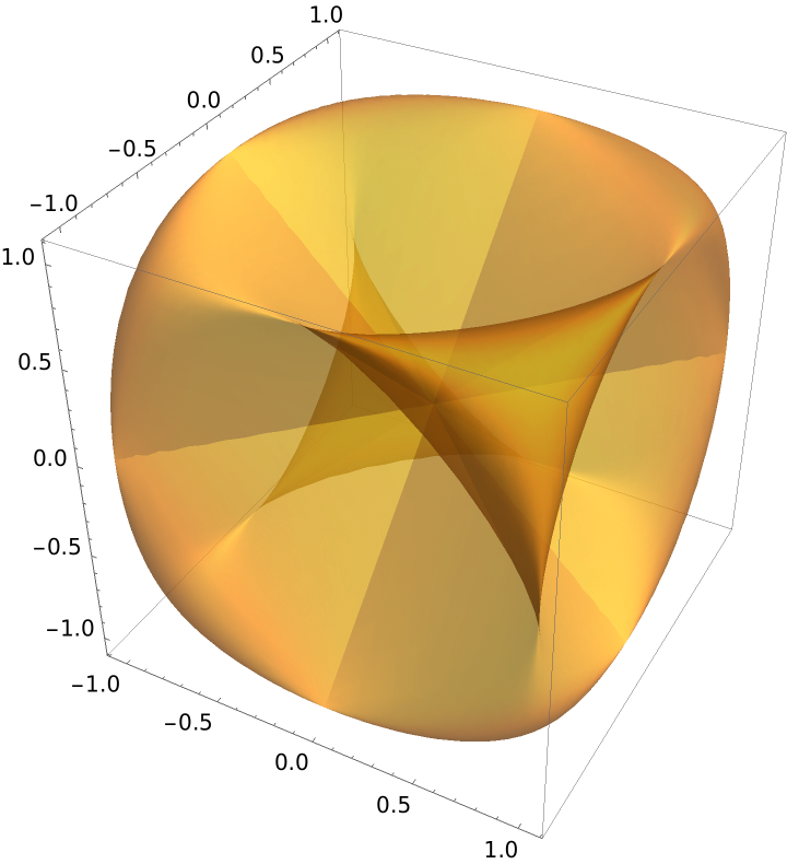 |
The parametrization of the unit normals of the sine surface:
| In[9]:= |
| Out[9]= |  |
A Gauss map shows where the normals "live" inside the unit sphere:
| In[10]:= | ![Show[Graphics3D[{Arrowheads[0.02], Arrow /@ Table[{{0, 0, 0}, normals /. u -> 1}, {v, 0.01, 2 \[Pi], 2 \[Pi]/40}], Opacity[.5], Sphere[]}], ParametricPlot3D[normals, {u, .8, 1.2}, {v, 0, 2 \[Pi]}, PlotStyle -> Opacity[.5], PlotPoints -> 40]]](https://www.wolframcloud.com/obj/resourcesystem/images/9f3/9f36e694-e56f-4026-b221-f6e9ec01bbe1/48823ecaa57c8833.png) |
| Out[10]= | 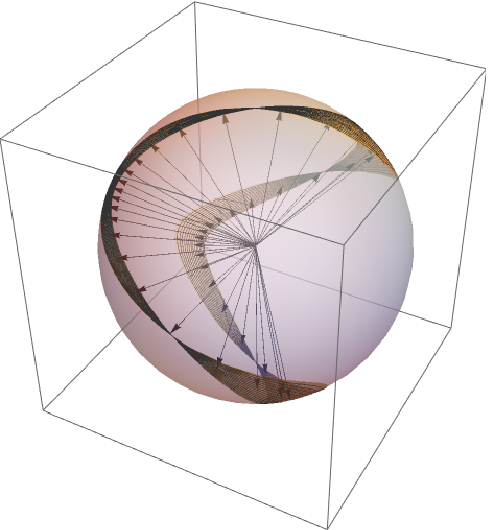 |
This work is licensed under a Creative Commons Attribution 4.0 International License