Details
Tsallis entropy is a generalization of the Boltzmann–Gibbs–Shannon entropy.
For a discrete set of probabilities
{pi}, the Tsallis entropy is defined as
.
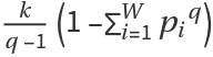
Tsallis entropy
Sq can equivalently be written as
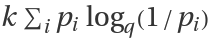
, or
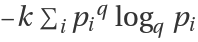
, or
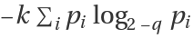
, where the
q-logarithm
logqz is defined as
logqz=(z1-q-1)/(1-q), with
log1z= log z being the limiting value as
q→1.
For a continuous probability distribution
p(x), the Tsallis entropy is defined as
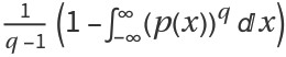
.
ResourceFunction["TsallisEntropy"][prob,q,k] computes the Tsallis entropy for a given discrete set of probabilities
prob={pi} with the condition
, where
W=Length[prob] is the number of possible configurations. If
prob is not normalized, it will be normalized first.
In the limit as q→1 for ResourceFunction["TsallisEntropy"][…], the Shannon differential entropy is recovered.
In ResourceFunction["TsallisEntropy"][prob,q,k], prob can be a list of real numbers. q and k can be real numbers.
In ResourceFunction["TsallisEntropy"][dist,q,k], dist can be any built-in continuous or discrete distribution in the Wolfram Language, or a mixture of them.
If not given, the default value of k is 1.
In ResourceFunction["TsallisEntropy"]["formula"], "formula" can be any of the following:
| "DiscreteFormula" | formula for Tsallis entropy for a discrete set of probabilities |
| "ContinuousFormula" | formula for Tsallis entropy for a continuous probability distribution |
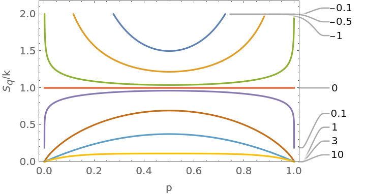
![Sq[p_] := Table[ResourceFunction["TsallisEntropy"][{p, 1 - p}, q, 1], {q, values = {-1, -0.5, -.1, 0, 0.1, 1, 3, 10}}];
Plot[Evaluate@Sq[p], {p, 0, 1}, PlotRange -> {0, 2}, FrameLabel -> {"p", "\!\(\*SubscriptBox[\(S\), \(q\)]\)/k"}, Frame -> True, PlotLabels -> values]](https://www.wolframcloud.com/obj/resourcesystem/images/448/44802a1e-c81e-4f54-97dd-095b62081f1b/118b51ab046befb1.png)
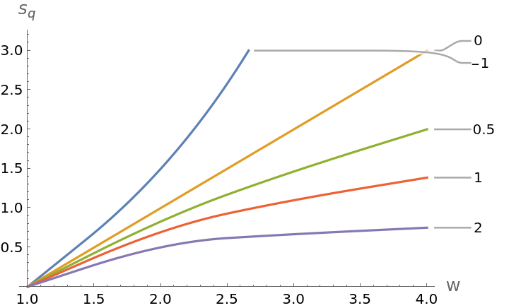
![ListPlot[Table[
ResourceFunction["TsallisEntropy"][Table[1/W, {x, 1, W}], q, 1], {q, {-1, 0, 0.5, 1, 2}}, {W, 1, 4}], Joined -> True, AxesOrigin -> {1, 0}, PlotRange -> {0, 3}, PlotLabels -> {-1, 0, 0.5, 1, 2}, InterpolationOrder -> 2, AxesLabel -> {"W", "\!\(\*SubscriptBox[\(S\), \(q\)]\)"}]](https://www.wolframcloud.com/obj/resourcesystem/images/448/44802a1e-c81e-4f54-97dd-095b62081f1b/71e22a0f2395ed10.png)
![q = 2;
p1 = {0.2, 0.3, 0.5};
p2 = {0.1, 0.6, 0.3};
ResourceFunction["TsallisEntropy"][Flatten@Outer[Times, p1, p2], q, 1] == ResourceFunction["TsallisEntropy"][p1, q, 1] + ResourceFunction["TsallisEntropy"][p2, q, 1] + (1 - q) ResourceFunction["TsallisEntropy"][p1, q, 1]*
ResourceFunction["TsallisEntropy"][p2, q, 1]](https://www.wolframcloud.com/obj/resourcesystem/images/448/44802a1e-c81e-4f54-97dd-095b62081f1b/056144a91b76254e.png)
![q = 1;
\[ScriptCapitalD]1 = NormalDistribution[0, 2];
\[ScriptCapitalD]2 = NormalDistribution[1/3, 1];
ResourceFunction["TsallisEntropy"][
ProductDistribution[\[ScriptCapitalD]1, \[ScriptCapitalD]2], q] == ResourceFunction["TsallisEntropy"][\[ScriptCapitalD]1, q] + ResourceFunction["TsallisEntropy"][\[ScriptCapitalD]2, q]](https://www.wolframcloud.com/obj/resourcesystem/images/448/44802a1e-c81e-4f54-97dd-095b62081f1b/61e81f26acc291d2.png)