Wolfram Function Repository
Instant-use add-on functions for the Wolfram Language
Function Repository Resource:
Evaluate the inverse of a tridiagonal matrix
ResourceFunction["TridiagonalInverse"][a,b,c] gives the inverse of the tridiagonal matrix with subdiagonal a, diagonal b and superdiagonal c. |
The inverse of a 3×3 tridiagonal matrix:
| In[1]:= |
| Out[1]= |  |
Multiply with the original tridiagonal matrix:
| In[2]:= | ![% . \!\(\*
TagBox[
RowBox[{"(", "", GridBox[{
{
SubscriptBox["b", "1"],
SubscriptBox["c", "1"], "0"},
{
SubscriptBox["a", "1"],
SubscriptBox["b", "2"],
SubscriptBox["c", "2"]},
{"0",
SubscriptBox["a", "2"],
SubscriptBox["b", "3"]}
},
GridBoxAlignment->{"Columns" -> {{Center}}, "Rows" -> {{Baseline}}},
GridBoxSpacings->{"Columns" -> {
Offset[
0.27999999999999997`], {
Offset[0.7]},
Offset[0.27999999999999997`]}, "Rows" -> {
Offset[0.2], {
Offset[0.4]},
Offset[0.2]}}], "", ")"}],
Function[BoxForm`e$,
MatrixForm[
SparseArray[
Automatic, {3, 3}, 0, {1, {{0, 2, 5, 7}, {{2}, {1}, {1}, {2}, {3}, {3}, {
2}}}, {Subscript[$CellContext`c, 1], Subscript[$CellContext`b, 1], Subscript[$CellContext`a, 1],
Subscript[$CellContext`b, 2], Subscript[$CellContext`c, 2], Subscript[$CellContext`b, 3],
Subscript[$CellContext`a, 2]}}]]]]\) // Simplify // MatrixForm](https://www.wolframcloud.com/obj/resourcesystem/images/dad/dadfb7fb-bbf6-43c6-8ce5-3f78b593704b/770b9e180b07e283.png) |
| Out[2]= |
TridiagonalInverse can be used with numerical entries:
| In[3]:= |
| Out[3]= |  |
| In[4]:= |
| Out[4]= |  |
Construct a natural cubic spline interpolant to data:
| In[5]:= | ![ya = {1., 2., 5., 7., 8., 5.};
n = Length[ya]; h = 0.5;
df = Differences[ya];
yp = ResourceFunction["TridiagonalInverse"][ConstantArray[1, n - 1], ArrayPad[ConstantArray[4, n - 2], 1, 2], ConstantArray[1, n - 1]] . (3/h Join[{df[[1]]}, ListConvolve[{1, 1}, df], {df[[-1]]}]);
iFun = Interpolation[Transpose[{List /@ (h Range[0, n - 1]), ya, yp}]]](https://www.wolframcloud.com/obj/resourcesystem/images/dad/dadfb7fb-bbf6-43c6-8ce5-3f78b593704b/2cebfec1591a3c91.png) |
| Out[5]= |
Plot the interpolant along with the data:
| In[6]:= |
| Out[6]= | 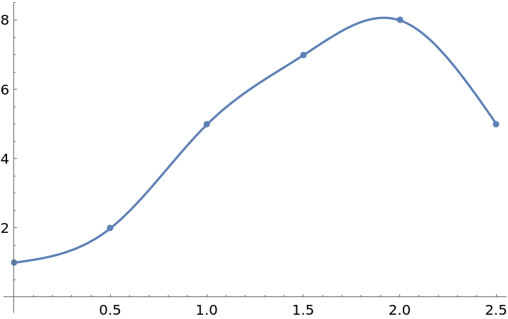 |
Approximately solve the boundary value problem u{XMLElement[span, {class -> stylebox}, {x, XMLElement[i, {class -> ti}, {x}]}]}+u=f;u(0)=u(1)=0:
| In[7]:= | ![f[x_] := Exp[-100 (x - 1/2)^2];
n = 100; h = 1./n; grid = N[Range[n - 1]]/n;
ux = ResourceFunction["TridiagonalInverse"][
ConstantArray[1/h^2, n - 2], ConstantArray[1. - 2/h^2, n - 1], ConstantArray[1/h^2, n - 2]] . (f[grid]);
ListPlot[Transpose[{grid, ux}]]](https://www.wolframcloud.com/obj/resourcesystem/images/dad/dadfb7fb-bbf6-43c6-8ce5-3f78b593704b/2ed69df98352e99d.png) |
| Out[7]= | 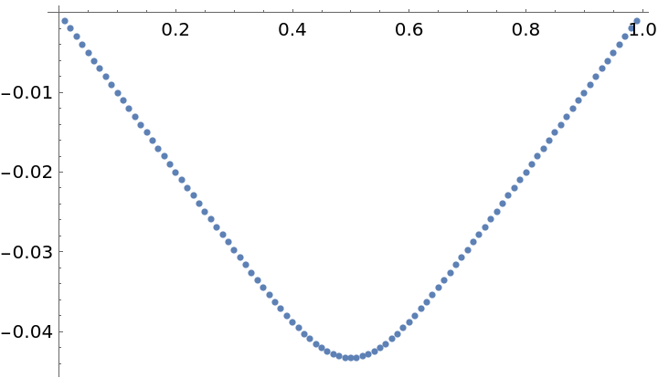 |
Show the error compared with the exact solution:
| In[8]:= |
| Out[8]= | 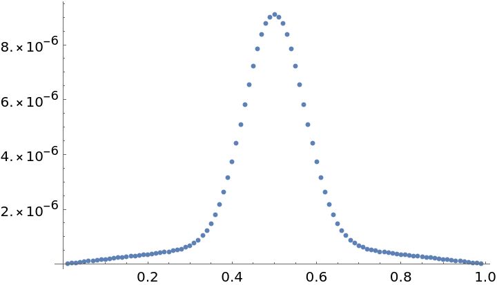 |
TridiagonalInverse can be faster than using Inverse on a tridiagonal matrix constructed with SparseArray and Band:
| In[9]:= | ![l1 = Table[
First[AbsoluteTiming[
With[{a = Array[\[Alpha], n - 1], b = Array[\[Beta], n], c = Array[\[Gamma], n - 1]},
Inverse[
SparseArray[{Band[{2, 1}] -> a, Band[{1, 1}] -> b, Band[{1, 2}] -> c}]]];]], {n, 3, 12}]; l2 = Table[First[
AbsoluteTiming[
With[{a = Array[\[Alpha], n - 1], b = Array[\[Beta], n], c = Array[\[Gamma], n - 1]}, ResourceFunction["TridiagonalInverse"][a, b, c]];]], {n, 3, 12}];](https://www.wolframcloud.com/obj/resourcesystem/images/dad/dadfb7fb-bbf6-43c6-8ce5-3f78b593704b/2780320c9292da33.png) |
| In[10]:= |
| Out[10]= | 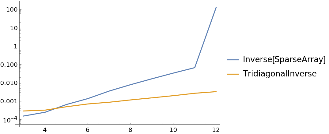 |
This work is licensed under a Creative Commons Attribution 4.0 International License