Function Repository Resource:

ThermodynamicBetheAnsatzSolve

Source Notebook

Solve integral equations of the thermodynamic Bethe ansatz type

Contributed by: Daniele Gregori

ResourceFunction["ThermodynamicBetheAnsatzSolve"][eqn]

solves a TBA equation.

ResourceFunction["ThermodynamicBetheAnsatzSolve"][eqn,y]

solves a TBA and returns the value of the solution.

ResourceFunction["ThermodynamicBetheAnsatzSolve"][{eqn₁,eqn₂, …}]

solves a system of TBA equations.

ResourceFunction["ThermodynamicBetheAnsatzSolve"][{eqn₁,eqn₂, …},{y₁,y₂,…}]

solves a system of TBA equations and returns the specified solutions values.

Details and Options

The Thermodynamic Bethe Ansatz (TBA) is a type of nonlinear integral equation studied extensively, in recent decades, in various branches of theoretical physics (especially in statistical field theory, quantum integrability and gauge theories).

Mathematically it has the following general form:

, where , for are the dependent variables, the non-homogeneous (or forcing) terms, the integral kernels (typically combinations of hyperbolic functions), some constants and . Notice that the integral terms are always convolutions.

Due to its quite involved form, the TBA cannot be solved analytically or symbolically through DSolve, but requires a special numerical treatment.

In particular, ResourceFunction["ThermodynamicBetheAnsatzSolve"] implements the method of successive approximations. In details, the solution is set first equal to the forcing terms, and then iterated in the equation until convergence is reached. Moreover, the convolutions are Fourier-transformed, then evaluated efficiently as products and transformed back through InverseFourier. To do this, the domain is discretized on a uniform finite grid and finally the solution is returned as an InterpolatingFunction object.

The first argument of ResourceFunction["ThermodynamicBetheAnsatzSolve"] is a TBA equation or a list of them. Then the solution is returned as a list of Rule expressions with an interpolating function solution for each dependent variable, in analogy with the output of NDSolve. The second argument, possibly empty, allows to return only the values of the solutions, in analogy with NDSolveValue.

ResourceFunction["ThermodynamicBetheAnsatzSolve"] accepts the following options:

"BoundaryCondition"

{0,0}

add boundary terms outside and inside the convolutions

"GridCutoff"

Automatic

specify the cutoff range of the numeric grid

"GridResolution"

2^10

specify the resolution of the numeric grid

"StoppingAccuracy"

10^(-10)

stop iterations when the numeric iteration error is lower than this value

MaxIterations

4000

always stop iterations beyond this value

"MonitorIterations"

False

monitor the number of iterations

"SaveMemory"

False

minimize caching to save memory

In principle, the numeric grid to obtain the solution, should have infinite cutoff (or range) and resolution. It is possible to simulate this ideal behaviour by giving increasingly values to the options "GridCutoff" and "GridResolution".

The iterations of the mathematical method of successive approximations are also in principle infinite and on the computer require a stopping rule. This can be simply a maximum limit on the iterations, as set by the option MaxIterations. Alternatively, they can be stopped even at a lower value, if the desired "StoppingAccuracy" error threshold is reached. This is defined, heuristically, as the maximum Norm difference, along all the grid, between the solution at a given iteration and the solution at the previous iteration.

The option "MonitorIterations" allows to Monitor the number of numeric iterations in real time and to then Echo the total number of iterations used.

By default, each numeric iteration is stored in the memory. This is not really necessary as to compute the next approximate solution only a single previous iteration is strictly required. So in some cases it may be desirable to use the option "SaveMemory" to use a special DataStructure["LeastRecentlyUsedCache"] to maintain inside the cache only the last iteration. This is not set as the default behaviour because it is found to lead also to a slightly lower speed.

For some special TBAs, further boundary conditions, besides the forcing terms, are required, either for specifying some further parameters or to improve accuracy. These boundary conditions are mathematically derived as terms to subtract to the forcing term and to the convolution integrand. They can be specified through the option "BoundaryCondition" as a list of two elements, or as a list of lists, if the TBA has multiple equations with different boundary conditions.

An "ansatz" is roughly translated as "educated guess." Alternates to the "thermodynamic" Bethe ansatz include algebraic, analytic, coordinate, functional and nested.

Examples

Basic Examples (2)

Solve a single non-linear integral equation, known as the "Sinh-Gordon" Thermodynamic Bethe Ansatz (TBA):

In[1]:=

$tbaSHG = y[x] == r Cosh[x] - \!$ \*SubsuperscriptBox[\(\[Integral]$, $-\[Infinity]$, $\[Infinity]$]$ \*FractionBox[\(Log[1 + \*SuperscriptBox[\(E$, $-y[t]$]]\ Sech[ t - x]\), $2\ \[Pi]$] \[DifferentialD]t\)\);$

In[2]:=

Out[2]=

Plot the solution:

In[3]:=

Out[3]=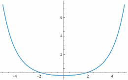

Scope (2)

Solve coupled non-linear integral equations, for example the TBA for the "pure SU(2) Seiberg-Witten" gauge theory:

In[4]:=

$(tbaSW0 = {y1[ x] == -2 E^ x \[Pi] (-1 + u/\[CapitalLambda]^2) Hypergeometric2F1[1/2, 1/2, 2, 1/2 (1 - u/\[CapitalLambda]^2)] - \!$ \*SubsuperscriptBox[\(\[Integral]$, $-\[Infinity]$, $\[Infinity]$]$ \*FractionBox[\(Log[1 + \*SuperscriptBox[\(E$, $-y2[t]$]]\ Sech[ t - x]\), $\[Pi]$] \[DifferentialD]t\)\), y2[x] == -2 E^ x \[Pi] (-1 - u/\[CapitalLambda]^2) Hypergeometric2F1[1/2, 1/2, 2, 1/2 (1 + u/\[CapitalLambda]^2)] - \!$ \*SubsuperscriptBox[\(\[Integral]$, $-\[Infinity]$, $\[Infinity]$]$ \*FractionBox[\(Log[1 + \*SuperscriptBox[\(E$, $-y1[t]$]]\ Sech[ t - x]\), $\[Pi]$] \[DifferentialD]t\)\)}) // Column$

Out[4]=

In[5]:=

$ResourceFunction["ThermodynamicBetheAnsatzSolve"][ tbaSW0 /. {u -> 1/10, \[CapitalLambda] -> 1}]$

Out[5]=

Plot the solutions:

In[6]:=

Out[6]=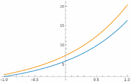

Solve the TBA for the "Perturbed Hairpin Integrable Model":

In[7]:=

$\[Phi]HP1[x_] := 1/(2 \[Pi]) Sqrt[3]/(2 Cosh[x] + 1) \[Phi]HP2[x_] := 1/(2 \[Pi]) Sqrt[3]/(2 Cosh[x] - 1) (tbaHP = {y1[ x] == (12 Sqrt[\[Pi]^3])/(Gamma[1/6] Gamma[1/3]) Exp[x] - 4/3 I \[Pi] q - \!$ \*SubsuperscriptBox[\(\[Integral]$, $-K$, $K$]$\[Phi]HP1[ x - t] Log[1 + Exp[\(-y1[t]$]] \[DifferentialD]t\)\) - \!$ \*SubsuperscriptBox[\(\[Integral]$, $-K$, $K$]$\[Phi]HP2[ x - t] Log[1 + Exp[\(-y2[t]$]] \[DifferentialD]t\)\), y2[x] == (12 Sqrt[\[Pi]^3])/(Gamma[1/6] Gamma[1/3]) Exp[x] + 4/3 I \[Pi] q - \!$ \*SubsuperscriptBox[\(\[Integral]$, $-K$, $K$]$\[Phi]HP1[ x - t] Log[1 + Exp[\(-y2[t]$]] \[DifferentialD]t\)\) - \!$ \*SubsuperscriptBox[\(\[Integral]$, $-K$, $K$]$\[Phi]HP2[ x - t] Log[ 1 + Exp[\(-y1[t]$]] \[DifferentialD]t\)\)}) // Column$

Out[8]=

Specify the parameter q, the integral cut-off K, and obtain the solution values:

In[9]:=

Out[9]=

Plot the real and imaginary parts of the solutions:

In[10]:=

Out[10]=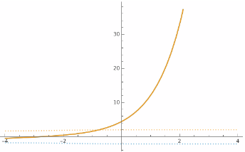

Options (17)

BoundaryCondition (6)

Some TBAs have to be solved with additional boundary conditions, required either for specifying additional physical parameters or for improving the convergence properties. For example, the TBA for the "Liouville Integrable Model" does not explicitly contain any parameter:

In[11]:=

$tbaLV = y[x] == (16 E^x \[Pi]^(3/2))/Gamma[1/4]^2 - \!$ \*SubsuperscriptBox[\(\[Integral]$, $-\[Infinity]$, $\[Infinity]$]$ \*FractionBox[\(Log[1 + \*SuperscriptBox[\(E$, $-y[t]$]]\ Sech[ t - x]\), $\[Pi]$] \[DifferentialD]t\)\);$

The solution can be computed anyway:

In[12]:=

Out[12]=

In[13]:=

Out[13]=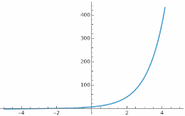

However, it is possible to specify a further physical parameter through the boundary condition for . To use in the TBA, it is first necessary to add to the forcing term an auxiliary function, with the same x→-∞ asymptotic behaviour as the boundary condition, and with zero limit for x → +∞, namely:

In[14]:=

In[15]:=

Out[15]=

In[16]:=

$Limit[bdyLVOut[P], x -> \[Infinity]]$

Out[16]=

Then, one must subtract the inverse convolution of this from the convolution integrand. That is:

In[17]:=

In[18]:=

$Convolve[bdyLVIn[P] /. x -> y, 1/\[Pi] Sech[y], y, x]$

Out[18]=

In[19]:=

Out[19]=

The TBA can now be solved for a series of parameters. P, specifying these external and internal boundary terms as option values:

In[20]:=

solBdyLV = Table[ResourceFunction["ThermodynamicBetheAnsatzSolve"][tbaLV, "BoundaryCondition" -> {bdyLVOut[P], bdyLVIn[P]}], {P, 0.5, 2., 0.5}]

Out[20]=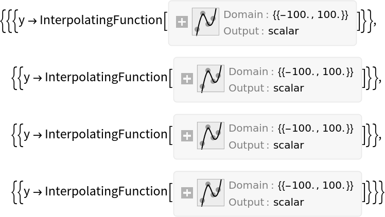

We can visualize these solutions and observe they have, as P→0, the solution with no boundary condition:

In[21]:=

$Plot[Values@Flatten@Prepend[solBdyLV, solLV] /. i_InterpolatingFunction :> i[x] // Evaluate, {x, -3, 3}, PlotLegends -> Prepend[Map["P = " <> ToString[#] &, Range[0.5, 2, 0.5]], "P = None"]]$

Out[21]=

GridCutoff (4)

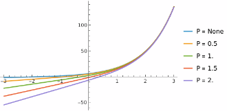By default, if the integration limits of the convolution are left specified symbolically as infinity, with numeric cut-offs set to :

In[22]:=

$ResourceFunction["ThermodynamicBetheAnsatzSolve"][ y[x] == r Cosh[x] - \!$ \*SubsuperscriptBox[\(\[Integral]$, $-\[Infinity]$, $\[Infinity]$]$ \*FractionBox[\(Log[1 + \*SuperscriptBox[\(E$, $-y[t]$]]\ Sech[ t - x]\), $2\ \[Pi]$] \[DifferentialD]t\)\) /. {r -> 0.1}, y]$

Out[22]=

The user can also specify different cut-offs by setting them directly in the equation:

In[23]:=

$ResourceFunction["ThermodynamicBetheAnsatzSolve"][ y[x] == r Cosh[x] - \!$ \*SubsuperscriptBox[\(\[Integral]$, $-K$, $K$]$ \*FractionBox[\(Log[1 + \*SuperscriptBox[\(E$, $-y[t]$]]\ Sech[ t - x]\), $2\ \[Pi]$] \[DifferentialD]t\)\) /. {r -> 0.1, K -> 20}, y]$

Out[23]=

Alternatively the numeric cut-off can be specified through the option "GridCutoff":

In[24]:=

Out[24]=

This option overrides the integration limits set inside the equation:

In[25]:=

Out[25]=

GridResolution (2)

Set up a TBA:

In[26]:=

$\[Phi]GHP[x_] := 1/(2 \[Pi] Cosh[x]) tbaGHP = {y1[x] == (8 Sqrt[\[Pi]^3])/Gamma[1/4]^2 Exp[x] - I \[Pi] (q1 - q2) - \!$ \*SubsuperscriptBox[\(\[Integral]$, $-K$, $K$]$\[Phi]GHP[ x - t] \((Log[1 + Exp[\(-y2[t]$]] + Log[1 + Exp[$-y3[t]$]])\) \[DifferentialD]t\)\), y2[x] == (8 Sqrt[\[Pi]^3])/Gamma[1/4]^2 Exp[x] - I \[Pi] (q1 + q2) - \!$ \*SubsuperscriptBox[\(\[Integral]$, $-K$, $K$]$\[Phi]GHP[ x - t] \((Log[1 + Exp[\(-y1[t]$]] + Log[1 + Exp[$-y4[t]$]])\) \[DifferentialD]t\)\), y3[x] == (8 Sqrt[\[Pi]^3])/Gamma[1/4]^2 Exp[x] + I \[Pi] (q1 + q2) - \!$ \*SubsuperscriptBox[\(\[Integral]$, $-K$, $K$]$\[Phi]GHP[ x - t] \((Log[1 + Exp[\(-y1[t]$]] + Log[1 + Exp[$-y4[t]$]])\) \[DifferentialD]t\)\), y4[x] == (8 Sqrt[\[Pi]^3])/Gamma[1/4]^2 Exp[x] + I \[Pi] (q1 - q2) - \!$ \*SubsuperscriptBox[\(\[Integral]$, $-K$, $K$]$\[Phi]GHP[ x - t] \((Log[1 + Exp[\(-y2[t]$]] + Log[1 + Exp[$-y3[t]$]])\) \[DifferentialD]t\)\)};$

By default, the integration interval is discretized into points. A finer grid, which can help with reaching higher numeric accuracy, can be achieved via the option "GridResolution":

In[27]:=

$ResourceFunction["ThermodynamicBetheAnsatzSolve"][ tbaGHP /. {q1 -> 0.2, q2 -> 0.3, K -> 50.}, "GridResolution" -> 2^12, "StoppingAccuracy" -> 10^(-15)]$

Out[27]=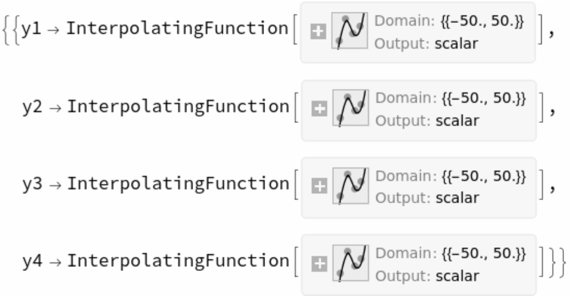

MonitorIterations (1)

Monitor the iterations in real time and Echo the total iterations used to obtain the numeric solution:

In[28]:=

$tbaSW0 = {y1[ x] == -2 E^ x \[Pi] (-1 + u/\[CapitalLambda]^2) Hypergeometric2F1[1/2, 1/2, 2, 1/2 (1 - u/\[CapitalLambda]^2)] - \!$ \*SubsuperscriptBox[\(\[Integral]$, $-\[Infinity]$, $\[Infinity]$]$ \*FractionBox[\(Log[1 + \*SuperscriptBox[\(E$, $-y2[t]$]]\ Sech[ t - x]\), $\[Pi]$] \[DifferentialD]t\)\), y2[x] == -2 E^ x \[Pi] (-1 - u/\[CapitalLambda]^2) Hypergeometric2F1[1/2, 1/2, 2, 1/2 (1 + u/\[CapitalLambda]^2)] - \!$ \*SubsuperscriptBox[\(\[Integral]$, $-\[Infinity]$, $\[Infinity]$]$ \*FractionBox[\(Log[1 + \*SuperscriptBox[\(E$, $-y1[t]$]]\ Sech[ t - x]\), $\[Pi]$] \[DifferentialD]t\)\)};$

In[29]:=

$ResourceFunction["ThermodynamicBetheAnsatzSolve"][ tbaSW0 /. {u -> 1/10, \[CapitalLambda] -> 1}, "MonitorIterations" -> True]$

Out[29]=

StoppingAccuracy (1)

Stop iterations when the (maximum norm) difference with the numeric solution at the previous iteration is below a certain threshold:

In[30]:=

In[31]:=

$ResourceFunction["ThermodynamicBetheAnsatzSolve"][ tbaSW0 /. {u -> 1/10, \[CapitalLambda] -> 1}, "MonitorIterations" -> True, "StoppingAccuracy" -> 10^(-8)]$

Out[31]=

As with a finer and larger grid, also a higher number of iteration usually leads a higher numeric accuracy.

MaxIterations (2)

Set a maximum number of iterations, which overrides the accuracy stopping rule:

In[32]:=

In[33]:=

$ResourceFunction["ThermodynamicBetheAnsatzSolve"][ tbaSW0 /. {u -> 1/10, \[CapitalLambda] -> 1}, "MonitorIterations" -> True, MaxIterations -> 500]$

Out[33]=

Setting a higher value for this option may be required to reach a lower stopping accuracy threshold:

In[34]:=

$ResourceFunction["ThermodynamicBetheAnsatzSolve"][ tbaSW0 /. {u -> 1/10, \[CapitalLambda] -> 1}, "MonitorIterations" -> True, "StoppingAccuracy" -> 10^(-14), MaxIterations -> 10^4]$

Out[34]=

SaveMemory (1)

Especially with very large TBAs (see the section "Neat Examples" below), or for finer grids or higher iterations, it can be convenient to use the "SaveMemory" option which maintains a cache of only the last iteration, instead of all of them:

In[35]:=

In[36]:=

$ResourceFunction["ThermodynamicBetheAnsatzSolve"][ tbaGHP /. {q1 -> 0.1, q2 -> 0.3, K -> 50.}, "GridResolution" -> 2^14, "StoppingAccuracy" -> 10^(-15), "SaveMemory" -> True]$

Out[36]=

Applications (13)

TBA modes (4)

The x → +∞ asymptotic expansion modes of the TBA solution are often related to physically interesting quantities. For example, consider the TBA for the "Liouville Integrable Model":

In[37]:=

$CLV[P_] := Log[(Gamma[2 P] Gamma[1 + 2 P])/(2 Pi)] bdyLV[P_] := {-8 P (Log[1 + Exp[-x]]) - CLV[P] (1 - Tanh[x/2]), -4 P Log[1 + Exp[-2 x]] - CLV[P] (1 - Tanh[x])} tbaLV = y[x] == (16 E^x \[Pi]^(3/2))/Gamma[1/4]^2 - \!$ \*SubsuperscriptBox[\(\[Integral]$, $-\[Infinity]$, $\[Infinity]$]$ \*FractionBox[\(Log[1 + \*SuperscriptBox[\(E$, $-y[t]$]]\ Sech[ t - x]\), $\[Pi]$] \[DifferentialD]t\)\)$

Out[38]=

Compute the first five asymptotic expansion modes of its convolution integral:

In[39]:=

$kernelModesLV[n_Integer] := Block[{vI, ker, unk, ser, coef, len, tab, thread, repl}, vI = x; ker = {-(Sech[x]/\[Pi])}; unk = Union@Flatten@ker; ser = Series[TrigToExp@unk /. vI -> Log@X, {X, \[Infinity], 2 n - 1}] // Normal; coef = CoefficientList[ser, 1/X]; tab = Map[Table[1/X^k, {k, 0, Length[#] - 1}] &, coef]; thread = MapThread[Times[#1, #2] &, {coef, tab}, 2]; repl = ker /. Normal@AssociationThread[unk, thread /. X -> Exp[vI]]] tbaModesLV[n_Integer] := Block[{vI, vInt, km, fL, thread}, vI = x; vInt = t; km = List@Map[PadRight[#, 2 n, 0] &, kernelModesLV[n], {1}]; fL = List@Map[Table[#, 2 n] &, {Log[1 + E^-y[t]]}, {1}]; thread = MapThread[Times[#1 /. vI -> vI - vInt, #2] &, {km, fL}, 3]; DeleteCases[Flatten@Map[MapApply[Plus, Transpose[#]] &, thread], 0]]$

In[40]:=

Out[40]=

Now solve the TBA equation:

In[41]:=

$solLV = With[{PP = 1}, ResourceFunction["ThermodynamicBetheAnsatzSolve"][tbaLV /. P -> PP, "BoundaryCondition" -> bdyLV[PP], "GridResolution" -> 2^12, "StoppingAccuracy" -> 10^(-12)]]$

Out[41]=

By integrating the TBA modes against this solution, one finds excellent agreement with the Liouville model integrals of motion (times a constant):

In[42]:=

$IMLV[1] = -(1/24) - P^2; IMLV[2] = 245/192 - 9/4 (1 - P^2) + (1 - P^2)^2; IMLV[3] = -(6675/3584) + 285/64 (1 - P^2) - 29/8 (1 - P^2)^2 + (1 - P^2)^3; IMLV[4] = 124025/36864 - 3605/384 (1 - P^2) + 4931/480 (1 - P^2)^2 - 31/6 (1 - P^2)^3 + (1 - P^2)^4; IMLV[5] = -(8665475/1081344) + (665955 (1 - P^2))/28672 - ( 52419 (1 - P^2)^2)/1792 + 627/32 (1 - P^2)^3 - 55/8 (1 - P^2)^4 + (1 - P^2)^5; Cn[n_] := Gamma[1/4 (-1 + 2 n)]^2/(2 Sqrt[\[Pi]] n!)$

In[43]:=

With[{PP = 1., nn = 5},
Prepend[
Transpose@{Splice@
Transpose@Table[{n, Cn[n] IMLV[n]} /. P -> PP, {n, nn}], Chop@NIntegrate[
tbaModesLV[nn] /. x -> 0 /. solLV[[1]], {t, -50, 50}]}, {"n", "IM (analytic)", "IM (TBA)"}]] // TableForm

Out[43]=

For more details, see reference[3].

ODE connection coefficients (9)

The TBA can be used to compute directly the connection coefficients of ordinary differential equations, in alternative to solving and integrating these.

Consider for example the Mathieu Ordinary Differential Equation:

In[44]:=

$odeMathieu = -\[HBar]^2 D[\[Psi][y], {y, 2}] + (\[CapitalLambda]^2 Cosh[y] + u) \[Psi][y] == 0$

Out[44]=

Map it into the corresponding Riccati equation:

In[45]:=

$riccatiMathieu = Simplify[ odeMathieu /. \[Psi] -> (Exp[ Integrate[\[ScriptCapitalP][#], #]] &)] /. Exp[_] :> 1$

Out[45]=

Compute its solution numerically and plot it:

In[46]:=

$riccatiMathieuSol[\[HBar]\[HBar]_, uu_, \[CapitalLambda]\[CapitalLambda]_, K_ : 12] := NDSolveValue[{riccatiMathieu, \[ScriptCapitalP][-K] == ( \[CapitalLambda] Sqrt[ Cosh[-K]])/\[HBar]} /. {\[HBar] -> \[HBar]\[HBar], u -> uu, \[CapitalLambda] -> \[CapitalLambda]\[CapitalLambda]}, \[ScriptCapitalP], {y, -K, K}]$

In[47]:=

$Plot[Evaluate@ Table[riccatiMathieuSol[\[HBar], 0.1, 1][y], {\[HBar], 0.1, 1.6, 0.3}], {y, -5, 5}, PlotLabels -> Table[\[HBar], {\[HBar], 0.1, 1.6, 0.3}], AxesLabel -> {y, \[ScriptCapitalP]}]$

Out[47]=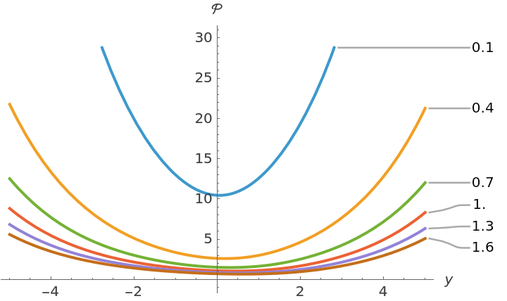

The logarithm of the central connection coefficient, called the Q function, is given as the regularized integral in the independent variable on the real line:

In[48]:=

$qRiccatiMathieu[\[HBar]_, u_, \[CapitalLambda]_, K_ : 10] := NIntegrate[ riccatiMathieuSol[\[HBar], u, \[CapitalLambda], K][y] - Sqrt[2] \[CapitalLambda] /\[HBar] Cosh[y/2], {y, -K, K}] qListMathieu[u_, \[CapitalLambda]_, K_ : 2, res_ : 0.1] := qListMathieu[u, \[CapitalLambda], K] = AssociationMap[qRiccatiMathieu[Exp[-#], u, \[CapitalLambda]] &, Range[-K, K, res]]$

We can compute it on a discretized grid of ℏ for various values of u:

In[49]:=

qLs1 = qListMathieu[0.1, 1];
qLs3 = qListMathieu[0.3, 1];
qLs5 = qListMathieu[0.5, 1];

Plot the resulting solution, for every :

In[50]:=

listPlotMathieu = ListPlot[
Map[List @@@ Normal@(Times[#, -2 Sqrt[2]] & /@ #) &, {qLs1, qLs3, qLs5}], PlotStyle -> Black, PlotMarkers -> {Automatic, Small}, AxesLabel -> {"x", "-2 ln Q"}]

Out[50]=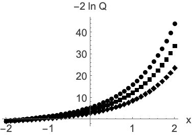

Now compare this connection coefficient with the solution of the "pure SU(2) Seiberg-Witten gauge theory" TBA, through the following map:

In[51]:=

$\[Phi]Nf0[x_] := 1/(2 \[Pi]) 2/Cosh[x] aDNf0[u_, \[CapitalLambda]_] := -I (u/\[CapitalLambda]^2 - 1)/ 2 Hypergeometric2F1[1/2, 1/2, 2, (1 - u/\[CapitalLambda]^2)/2] tbaNf0 = {y1[x] == -4 \[Pi] I aDNf0[u, \[CapitalLambda]] Exp[x] - \!$ \*SubsuperscriptBox[\(\[Integral]$, $-K$, $K$]$\[Phi]Nf0[ x - t] Log[1 + Exp[\(-y2[t]$]] \[DifferentialD]t\)\), y2[x] == -4 \[Pi] I aDNf0[-u, \[CapitalLambda]] Exp[x] - \!$ \*SubsuperscriptBox[\(\[Integral]$, $-K$, $K$]$\[Phi]Nf0[ x - t] Log[1 + Exp[\(-y1[t]$]] \[DifferentialD]t\)\)}; bdyNf0 = {-2 Log[ 1 + 2/\[Pi] Log[1 + Exp[-x ]]], -Log[ 1 + 2/\[Pi] Log[1 + I Exp[-x ]]] - Log[1 + 2/\[Pi] Log[1 - I Exp[-x ]]]};$

In[52]:=

$tbaNf0sol = Table[ResourceFunction["ThermodynamicBetheAnsatzSolve"][ tbaNf0 /. {u -> uu, \[CapitalLambda] -> 1}, y1, "BoundaryCondition" -> bdyNf0], {uu, 0.1, 0.5, 0.2}]$

Out[52]=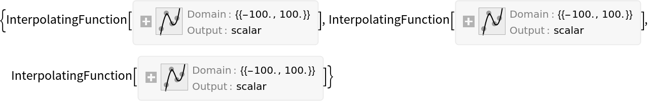

Plot the solution of TBA:

In[53]:=

$plotNf0 = Plot[tbaNf0sol /. i_InterpolatingFunction :> i[x] // Evaluate, {x, -2, 2}, PlotRange -> All, PlotLabels -> {0.1, 0.3, 0.5}, AxesLabel -> {x, y1}]$

Out[53]=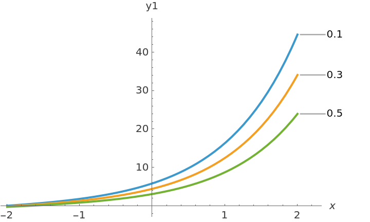

The plot perfectly matches that of the connection coefficient of the Mathieu equation:

In[54]:=

Out[54]=

For more details, see reference[3] and arXiv:2208.14031-revised.pdf.

Properties and Relations (8)

TBA equivalence (8)

Different TBA equations may actually describe the same solution, in different variables.

For example consider the TBAs for the "Perturbed Hairpin Integrable Model" and the "1-flavour SU(2) Seiberg-Witten gauge theory", defined as follows:

In[55]:=

$\[Phi]HP1[x_] := 1/(2 \[Pi]) Sqrt[3]/(2 Cosh[x] + 1) \[Phi]HP2[x_] := 1/(2 \[Pi]) Sqrt[3]/(2 Cosh[x] - 1) tbaHP = {y1[x] == (12 Sqrt[\[Pi]^3])/(Gamma[1/6] Gamma[1/3]) Exp[x] - 4/3 I \[Pi] q - \!$ \*SubsuperscriptBox[\(\[Integral]$, $-K$, $K$]$\[Phi]HP1[ x - t] Log[1 + Exp[\(-y1[t]$]] \[DifferentialD]t\)\) - \!$ \*SubsuperscriptBox[\(\[Integral]$, $-K$, $K$]$\[Phi]HP2[ x - t] Log[1 + Exp[\(-y2[t]$]] \[DifferentialD]t\)\), y2[x] == (12 Sqrt[\[Pi]^3])/(Gamma[1/6] Gamma[1/3]) Exp[x] + 4/3 I \[Pi] q - \!$ \*SubsuperscriptBox[\(\[Integral]$, $-K$, $K$]$\[Phi]HP1[ x - t] Log[1 + Exp[\(-y2[t]$]] \[DifferentialD]t\)\) - \!$ \*SubsuperscriptBox[\(\[Integral]$, $-K$, $K$]$\[Phi]HP2[ x - t] Log[1 + Exp[\(-y1[t]$]] \[DifferentialD]t\)\)}; CHP[P_, q_] := Log[(Gamma[2 P] Gamma[1 + 2 P])/( 2^P Sqrt[2 Pi] Sqrt[Gamma[1/2 + q + P] Gamma[1/2 - q + P]])] bdyHP[P_, q_] := {-3 P (Log[1 + Exp[-x - I \[Pi]/6]] + Log[1 + Exp[-x + I \[Pi]/6]]) - CHP[P, q] (1 - 1/2 Tanh[x/2 + I \[Pi]/12] - 1/2 Tanh[x/2 - I \[Pi]/12]), -3 P Log[1 + Exp[-2 x]] - CHP[P, q] (1 - Tanh[x])}$

In[56]:=

$\[Phi]pNf1[x_] := 1/(2 \[Pi] Cosh[x + I \[Pi]/6]) \[Phi]mNf1[x_] := 1/(2 \[Pi] Cosh[x - I \[Pi]/6]) lQ0Nf1[u_, m_, \[CapitalLambda]_] := With[{N = 30}, Sum[((4 m)/\[CapitalLambda])^n ((4 u)/\[CapitalLambda]^2)^ l Binomial[1/2, n] Binomial[1/2 - n, l] If[n == 1 && l == 0, 2 Log[2]/3, 1/3 Beta[1/6 (2 l + 4 n - 1), 1/3 (2 l + n - 1)]], {n, 0, N}, {l, 0, N}]]; eps0Nf1[k_, u_, m_, \[CapitalLambda]_] := -Exp[-I \[Pi]/6] lQ0Nf1[ Exp[I \[Pi]/3] Exp[2 \[Pi] I k/3] u, Exp[ \[Pi] I/6] Exp[-2 \[Pi] I k/3] m, \[CapitalLambda]] - Exp[I \[Pi]/6] lQ0Nf1[ Exp[-I \[Pi]/3] Exp[ 2 \[Pi] I k/3] u, -Exp[ -\[Pi] I/6] Exp[-2 \[Pi] I k/ 3] m, \[CapitalLambda]] - I 8/3 \[Pi] Exp[-2 \[Pi] I k/3] m/\[CapitalLambda]; tbaNf1 := {yp0[x] == eps0Nf1[0, u, m, \[CapitalLambda]] Exp[x] - \!$ \*SubsuperscriptBox[\(\[Integral]$, $-K$, $K$]$\[Phi]pNf1[ x - t] Log[ 1 + Exp[\(-yp1[t]$]] \[DifferentialD]t\)\) - \!$ \*SubsuperscriptBox[\(\[Integral]$, $-K$, $K$]$\[Phi]mNf1[ x - t] Log[1 + Exp[\(-yp2[t]$]] \[DifferentialD]t\)\), yp1[x] == eps0Nf1[1, u, m, \[CapitalLambda]] Exp[x] - \!$ \*SubsuperscriptBox[\(\[Integral]$, $-K$, $K$]$\[Phi]pNf1[ x - t] Log[ 1 + Exp[\(-yp2[t]$]] \[DifferentialD]t\)\) - \!$ \*SubsuperscriptBox[\(\[Integral]$, $-K$, $K$]$\[Phi]mNf1[ x - t] Log[1 + Exp[\(-yp0[t]$]] \[DifferentialD]t\)\), yp2[x] == eps0Nf1[2, u, m, \[CapitalLambda]] Exp[x] - \!$ \*SubsuperscriptBox[\(\[Integral]$, $-K$, $K$]$\[Phi]pNf1[ x - t] Log[ 1 + Exp[\(-yp0[t]$]] \[DifferentialD]t\)\) - \!$ \*SubsuperscriptBox[\(\[Integral]$, $-K$, $K$]$\[Phi]mNf1[ x - t] Log[ 1 + Exp[\(-yp1[ t]$]] \[DifferentialD]t\)\)} /. \[CapitalLambda] -> 1; bdyNf1 = -{Log[1 + 2/\[Pi] Log[1 + Exp[-x - I \[Pi]/6]]] + Log[1 + 2/\[Pi] Log[1 + Exp[-x + I \[Pi]/6]]], Log[1 + 2/\[Pi] Log[1 + I Exp[-x ]]] + Log[1 + 2/\[Pi] Log[1 - I Exp[-x ]]]};$

These TBA equations appear as very different in structure:

In[57]:=

Out[57]=

In[58]:=

$Block[{Sum = Inactive[Sum]}, tbaNf1 /. S : Inactive[Sum][__] :> Magnify[S, 0.6]] // Column$

Out[58]=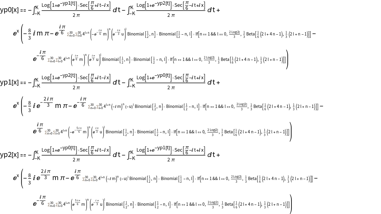

However, as explained in reference[4] - see also its revised version at arXiv:2208.14031-revised.pdf - the two TBAs actually have the same solution, under the following change of parameters:

The rules for changing parameters from one model to the other and vice-versa, are simply obtained by solving these equations for p and q in terms of u and m, at any x:

In[59]:=

$ruleParNf1GauInt[xx_, u_, m_] := Join[{x -> xx}, Last@Solve[{u == 1/4 p^2 Exp[-2 xx], m == 1/2 q Exp[-xx]}, {p, q}]] ruleParNf1IntGau[xx_, p_, q_] := Join[{x -> xx}, Last@Solve[{u == 1/4 p^2 Exp[-2 xx], m == 1/2 q Exp[-xx]}, {u, m}]]$

For example, fix the parameters u=0.1, m=0.05 ⅈ, find their corresponding p,q parameters for x∈{-1,0,1,2,3}, and solve the Perturbed Hairpin equations:

In[60]:=

tbaHPListEquiv = With[{u = 0.1, m = 0.05 I, xL = Range[-1, 3]}, MapApply[#1 -> ResourceFunction["ThermodynamicBetheAnsatzSolve"][
tbaHP /. Join[{q -> #3, p -> #2}, {K -> 40}], y1, "BoundaryCondition" -> bdyHP[#2, #3]] &, Values@ruleParNf1GauInt[#, u, m] & /@ xL]] // Association

Out[60]=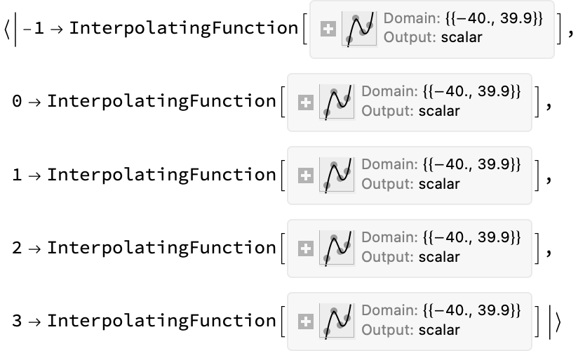

It turns out that, at each x, these "Perturbed Hairpin" TBA solutions match precisely the solution of the other "1-flavor gauge theory" TBA, for chosen parameters u=0.1, m=0.05 ⅈ:

In[61]:=

Out[61]=

A combined plot shows such equivalence:

In[62]:=

$plotEquivNf1GauInt = Block[{pars = {1/10, 1/20 }, colors, legends, sols, style, epilog, plot, listplot}, colors = Take[ColorData["DefaultPlotColors", "ColorList"], 5]; legends = MapApply["p=" <> ToString@N@#1 <> ", q=" <> ToString@N@#2 <> "i" &, Map[Values@Take[#, -2] &, ruleParNf1GauInt[#, Sequence @@ pars] & /@ Range[-1, 3] // MapAt[NumberForm[#, 5] &, #, {All, All, 2}] &]]; sols = Join[{tbaNf1RefEquiv}, Values@tbaHPListEquiv] /. i_InterpolatingFunction :> i[x]; style = {Black, Sequence @@ Map[{#, Dashed} &, colors]}; epilog = MapIndexed[{PointSize[Large], colors[[#2[[1]]]], Point[{#1, tbaNf1RefEquiv[#1]}]} &, Range[-1, 3]]; listplot = ListPlot[ Map[List@ Callout[{#, Chop@tbaNf1RefEquiv[#]}, NumberForm[{#, Chop@tbaNf1RefEquiv[#]}, 5], {Above, Right}] &, Range[-1, 3]], PlotStyle -> PointSize[Large]]; plot = Plot[sols, {x, -2, 4}, PlotStyle -> style, Epilog -> epilog, PlotLegends -> {"u=0.1, m=0.05i", Sequence @@ legends}, AxesLabel -> {x, y[x]}]; Show[plot, listplot, ImageSize -> 500]]$

Out[62]=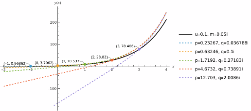

Of course, the argument could be inverted, namely one could fix the p,q parameters, solve the Perturbed Hairpin TBA, and find a match with the solutions of the 1-flavour gauge theory TBA, with the corresponding u,m parameters, at any fixed x. For more details, see arXiv:2208.14031-revised.pdf.

Possible Issues (2)

Only numerical solutions of the TBA, for special values of the parameters, can be provided:

In[63]:=

In[64]:=

Out[64]=

The behaviour under change of parameters should then be investigated through multiple TBA solutions:

In[65]:=

Out[65]=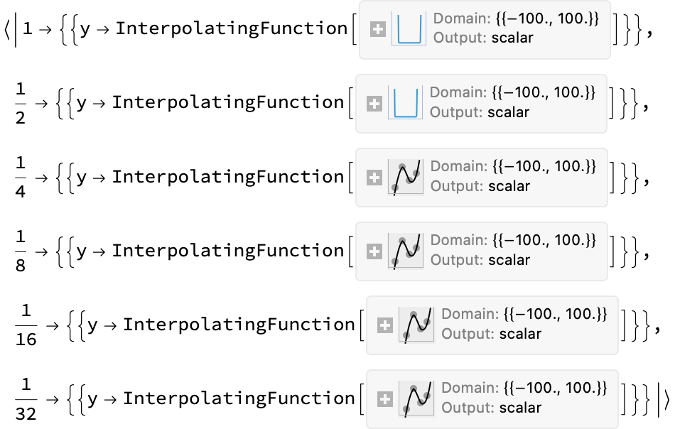

In[66]:=

Plot[y[x] /. Flatten[Values@solsR, 1] // Evaluate, {x, -3, 3}, PlotLegends -> Map[StringJoin["r = ", ToString[#]] &, N@Keys[solsR]],
PlotStyle -> Map[Hue, Range[1/3, 3/4, 1/12]], AxesLabel -> {x, y[x, r]}]

Out[66]=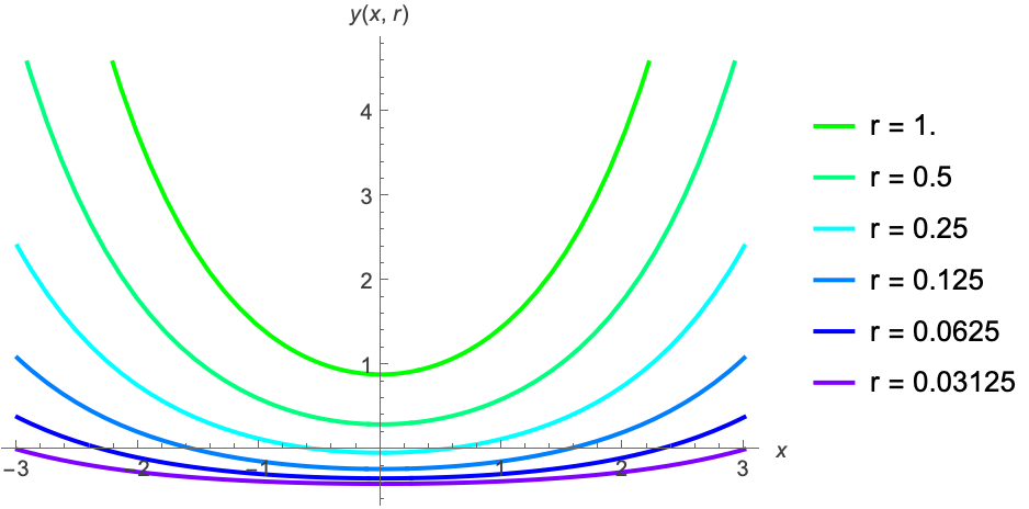

TBA equations are typically defined only in certain regions of the parameter space, outside which they are non-convergent:

In[67]:=

$\[Phi]Nf0[x_] := 1/(2 \[Pi]) 2/Cosh[x] aDNf0[u_, \[CapitalLambda]_] := -I (u/\[CapitalLambda]^2 - 1)/ 2 Hypergeometric2F1[1/2, 1/2, 2, (1 - u/\[CapitalLambda]^2)/2] tbaNf0 = {y1[x] == -4 \[Pi] I aDNf0[u, \[CapitalLambda]] Exp[x] - \!$ \*SubsuperscriptBox[\(\[Integral]$, $-\[Infinity]$, $\[Infinity]$]$\[Phi]Nf0[x - t] Log[ 1 + Exp[\(-y2[t]$]] \[DifferentialD]t\)\), y2[x] == -4 \[Pi] I aDNf0[-u, \[CapitalLambda]] Exp[x] - \!$ \*SubsuperscriptBox[\(\[Integral]$, $-\[Infinity]$, $\[Infinity]$]$\[Phi]Nf0[x - t] Log[ 1 + Exp[\(-y1[t]$]] \[DifferentialD]t\)\)};$

In[68]:=

$ResourceFunction["ThermodynamicBetheAnsatzSolve"][ tbaNf0 /. {u -> 2, \[CapitalLambda] -> 1}]$

Out[68]=

In this case, we can easily understand why: the forcing terms become non-positive outside the segment u ∈ [-Λ^2,+Λ^2]:

In[69]:=

$Table[{N@u, 1, Splice@Map[ N[#, 3] &, {-4 \[Pi] I aDNf0[u, 1], -4 \[Pi] I aDNf0[-u, 1]}]}, {u, -2, 2, 1/2}] // Tabular[#, {"u", "\[CapitalLambda]", "forc. term. 1", "forc. term. 2"}, ImageSize -> {All, All}, AppearanceElements -> {"ColumnHeaders"}, Background -> <| "RowValueFunction" -> Function@ If[Or[Re[#"forc. term. 1"] < 0, Re[#"forc. term. 2"] < 0], LightDarkSwitched[LightRed], None]|>] &$

Out[69]=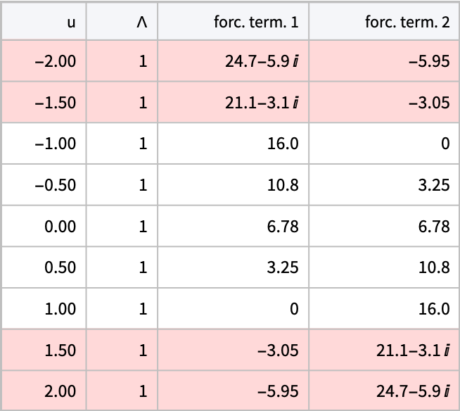

Visualize the convergence region also for complex u:

In[70]:=

$Block[{plotReRe, plotPlane, plotConts, R = 2}, plotReRe = Plot3D[Re[-4 \[Pi] I aDNf0[ru + I iu, 1]] Re[-4 \[Pi] I aDNf0[-ru - I iu, 1]], {ru, -R, R}, {iu, -R, R}, ColorFunction -> "SolarColors", AxesLabel -> {"Re[u]", "Im[u]"}, PlotRange -> {-100, 50}]; plotPlane = Plot3D[0, {ru, -R, R}, {iu, -R, R}, PlotStyle -> {StandardBlue, Opacity[0.5]}, Mesh -> None]; plotConts = ContourPlot3D[{Re[-4 \[Pi] I aDNf0[ru + I iu, 1]] == 0, Re[-4 \[Pi] I aDNf0[-ru - I iu, 1]] == 0}, {ru, -R, R}, {iu, -R, R}, {z, -0.5, 0.5}, ContourStyle -> Black, Mesh -> None]; Show[plotReRe, plotPlane, plotConts]]$

Out[70]=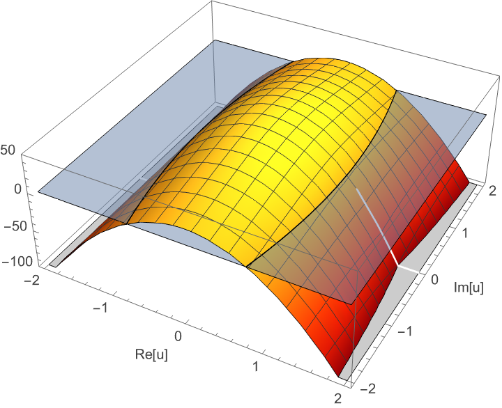

Then, iterating this forcing term in the equation (by the method of successive approximations), clearly leads to divergent convolution integrals (due to the divergent double exponentials in the integrands). Some techniques exist to analytically continue the TBA equations and make them always convergent (in principle following the so-called Y systems), but they are outside the scope of this resource.

Neat Examples (5)

The previous examples showed relatively simple systems of TBA equations. Instead, the following is a much more complex TBA, with an arbitrary number of equations:

In[71]:=

$\[Chi][a_, x_] := 2/\[Pi] (Cos[(a \[Pi])/2] Cosh[x])/(Cos[a \[Pi]] + Cosh[2 x]) \[Psi][a_, x_] := 1/\[Pi] Sin[a \[Pi]]/(Cos[a \[Pi]] + Cosh[2 x]) \[Phi][a_, x_] := 1/(2 \[Pi]) a/Cosh[a x] tbaFFPT[p_] := tbaFFPT[p] = Block[{A}, A[_, i_, j_] := KroneckerDelta[i, j + 1] + KroneckerDelta[i, j - 1]; Union@Join[{y0[x] == m R Cosh[x] + I \[Alpha] - 1/2 Sum[\!$ \*SubsuperscriptBox[\(\[Integral]$, $-K$, $K$]$\[Chi][ 1 - 2 l/4, x - t] Log[ 1 + Exp[\(Symbol["\<y\>" <> ToString@l <> "\<a1\>"]$[ t]]] \[DifferentialD]t\)\), {l, 1, 3}] - 1/2 Sum[\!$ \*SubsuperscriptBox[\(\[Integral]$, $-K$, $K$]$\[Psi][ 1 - 2 l/4, x - t] Log[ 1 + Exp[\(Symbol["\<y\>" <> ToString@l <> "\<a1\>"]$[ t]]] \[DifferentialD]t\)\), {l, 1, 3}], y0b[x] == m R Cosh[x] - I \[Alpha] - 1/2 Sum[\!$ \*SubsuperscriptBox[\(\[Integral]$, $-K$, $K$]$\[Chi][ 1 - 2 l/4, x - t] Log[ 1 + Exp[\(Symbol["\<y\>" <> ToString@l <> "\<a1\>"]$[ t]]] \[DifferentialD]t\)\), {l, 1, 3}] + 1/2 Sum[\!$ \*SubsuperscriptBox[\(\[Integral]$, $-K$, $K$]$\[Psi][ 1 - 2 l/4, x - t] Log[ 1 + Exp[\(Symbol["\<y\>" <> ToString@l <> "\<a1\>"]$[ t]]] \[DifferentialD]t\)\), {l, 1, 3}]}, Flatten@ Table[Symbol["y" <> ToString[i] <> "a" <> ToString[j]][x] == KroneckerDelta[i, 1] KroneckerDelta[j, 1] \!$ \*SubsuperscriptBox[\(\[Integral]$, $-K$, $K$]$\[Phi][2, x - t] Log[1 + Exp[\(-y0[t]$]] \[DifferentialD]t\)\) + KroneckerDelta[i, 3] KroneckerDelta[j, 1] \!$ \*SubsuperscriptBox[\(\[Integral]$, $-K$, $K$]$\[Phi][2, x - t] Log[1 + Exp[\(-y0b[t]$]] \[DifferentialD]t\)\) + Sum[A[\[Infinity], l, j] \!$ \*SubsuperscriptBox[\(\[Integral]$, $-K$, $K$]$\[Phi][2, x - t] Log[ 1 + Exp[\(Symbol["\<y\>" <> ToString@i <> "\<a\>" <> ToString@l]$[t]]] \[DifferentialD]t\)\), {l, 1, p - 1}] - Sum[A[3, l, i] \!$ \*SubsuperscriptBox[\(\[Integral]$, $-K$, $K$]$\[Phi][2, x - t] Log[ 1 + Exp[\(-\(Symbol["\<y\>" <> ToString@l <> "\<a\>" <> ToString@j]$[t]\)]] \[DifferentialD]t\)\), {l, 1, 3}], {i, 1, 3}, {j, 1, p - 1}]]];$

For example, with parameter p=10, the TBA is modeled by the following 29 coupled equations:

In[72]:=

Out[72]=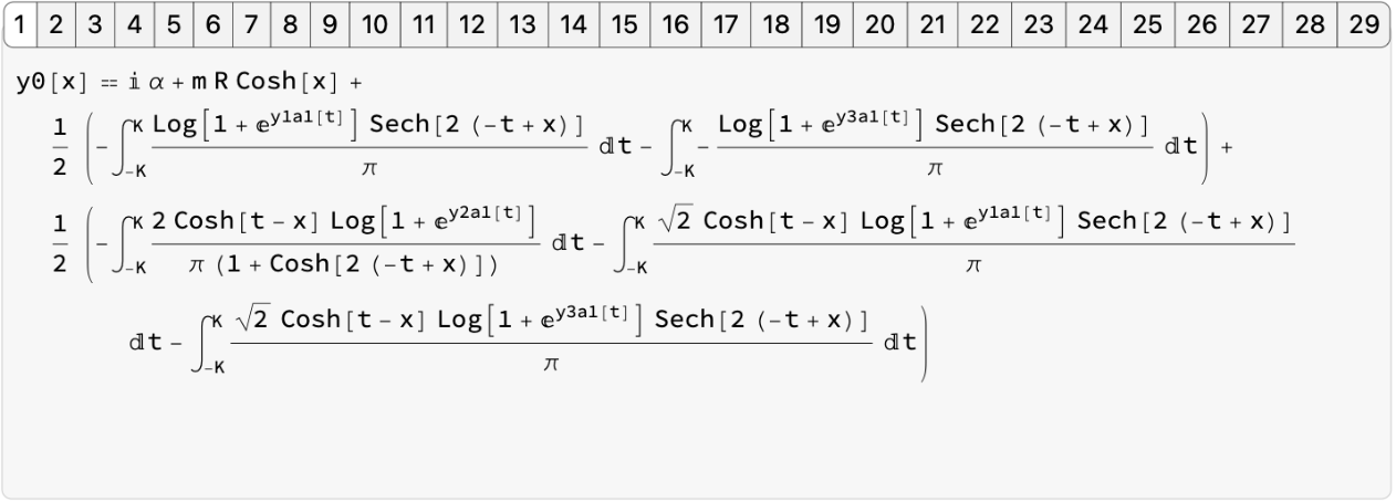

The following integral of the TBA solution, called central charge, is a physically interesting quantity:

In[73]:=

$centralCharge[p_, mm_, RR_, \[Alpha]\[Alpha]_, KK_ : 20, options : OptionsPattern[]] := Block[{sol}, sol = ResourceFunction["ThermodynamicBetheAnsatzSolve"][ tbaFFPT[p] /. {m -> mm, R -> RR, K -> KK, \[Alpha] -> \[Alpha]\[Alpha]}, options]; 3 mm RR/\[Pi]^2 NIntegrate[ Cosh[t] (Log[1 + E^-y0[t]] + Log[1 + E^-y0b[t]]) /. sol, {t, -KK, KK}][[1]]]$

Let us compute it for increasingly larger p and compare it with its known analytic limit for :

In[74]:=

We reproduce the results of reference[2]:

In[75]:=

$ParallelTable[ {p, centralChargeLimit[p], centralCharge[p, 1*10^(-17), 1*10^(-17), 0, 600, "GridResolution" -> 2^14, "SaveMemory" -> True] // Quiet}, {p, 2, 41, 3}] // Prepend[#, {"p", "cent. charge (analytic)", "cent. charge (TBA)"}] & // TableForm$

Out[75]=

Publisher

Daniele Gregori

Requirements

Wolfram Language 12.1 (March 2020) or above

Version History

1.0.0 – 22 September 2025

Source Metadata

Citation:
- [1] A. B. Zamolodchikov, "Thermodynamic Bethe Ansatz in Relativistic Models. Scaling Three State Potts and Lee-yang Models", Nucl. Phys. B 342 (1990), 695-720, doi:10.1016/0550-3213(90)90333-9
- [2] A. Fabbri, D. Fioravanti, S. Piscaglia and R. Tateo, "Exact results for the low energy $AdS_4$ x $\mathbb{CP}^3$ string theory", JHEP 11 (2013), 073, doi:10.1007/JHEP11(2013)073, arXiv:1308.1861[hep-th]
- [3] D. Fioravanti, D. Gregori, "Integrability and cycles of deformed ${\cal N}=2$ gauge theory'', Phys. Lett. B 804 (2020), 135376 doi:10.1016/j.physletb.2020.135376, arXiv:1908.08030[hep-th]
- [4] D. Fioravanti, D. Gregori and H. Shu, "Integrability, susy $SU(2)$ matter gauge theories and black holes", arXiv:2208.14031[hep-th]

Related Resources

Author Notes

A small part of this code, for solving particular TBA equations, I initially learned from my collaborator Prof. Hongfei Shu, but I essentially improved it and generalized it into an actual package which can automatically solve any TBA.

License Information

This work is licensed under a Creative Commons Attribution 4.0 International License

Wolfram Function Repository

ThermodynamicBetheAnsatzSolve

Details and Options

Examples

Basic Examples (2)

Scope (2)

Options (17)

BoundaryCondition (6)

GridCutoff (4)

GridResolution (2)

MonitorIterations (1)

StoppingAccuracy (1)

MaxIterations (2)

SaveMemory (1)

Applications (13)

TBA modes (4)

ODE connection coefficients (9)

Properties and Relations (8)

TBA equivalence (8)

Possible Issues (2)

Neat Examples (5)

Publisher

Related Links

Requirements

Version History

Source Metadata

Related Resources

Author Notes

License Information

ThermodynamicBetheAnsatzSolve

Details and Options

Examples

Basic Examples (2)

Scope (2)

Options (17)

BoundaryCondition (6)

GridCutoff (4)

GridResolution (2)

MonitorIterations (1)

StoppingAccuracy (1)

MaxIterations (2)

SaveMemory (1)

Applications (13)

TBA modes (4)

ODE connection coefficients (9)

Properties and Relations (8)

TBA equivalence (8)

Possible Issues (2)

Neat Examples (5)

Publisher

Related Links

Requirements

Version History

Source Metadata

Related Resources

Related Symbols

Author Notes

License Information