Wolfram Function Repository
Instant-use add-on functions for the Wolfram Language
Function Repository Resource:
Transform components of tensors with arbitrary rank with regard to their transformation behavior under any given mapping
ResourceFunction["TensorCoordinateTransform"][tensor,mat] transform tensor components according to their transformation behavior matrix mat. All tensor slots are considered to be contravariant and not normalized. |
| "TransformationBehavior" | "AllContravariant" | transformation behavior of individual components |
| "Normalize" | False | whether the components are represented with respect to a normalized basis |
Apply a rotation transformation to a tensor:
| In[1]:= | ![ResourceFunction[
"TensorCoordinateTransform"][{Subscript[v, 1], Subscript[v, 2], Subscript[v, 3]}, ( {
{Cos[\[Phi]], -Sin[\[Phi]], 0},
{Sin[\[Phi]], Cos[\[Phi]], 0},
{0, 0, 1}
} )]](https://www.wolframcloud.com/obj/resourcesystem/images/6d0/6d084720-3979-4be8-9075-48fe6c7d9d7f/793e9887df008161.png) |
| Out[1]= |
Rotate vector components about the three axes counterclockwise:
| In[2]:= | ![ResourceFunction[
"TensorCoordinateTransform"][{Subscript[v, 1], Subscript[v, 2], Subscript[v, 3]}, ( {
{Cos[\[Phi]], -Sin[\[Phi]], 0},
{Sin[\[Phi]], Cos[\[Phi]], 0},
{0, 0, 1}
} )] // Simplify // MatrixForm](https://www.wolframcloud.com/obj/resourcesystem/images/6d0/6d084720-3979-4be8-9075-48fe6c7d9d7f/282d0a2e46e0142e.png) |
| Out[2]= |
Change the axis:
| In[3]:= | ![ResourceFunction[
"TensorCoordinateTransform"][{Subscript[v, 1], Subscript[v, 2], Subscript[v, 3]}, ( {
{0, 1, 0},
{0, 0, 1},
{1, 0, 0}
} )] // MatrixForm](https://www.wolframcloud.com/obj/resourcesystem/images/6d0/6d084720-3979-4be8-9075-48fe6c7d9d7f/3e6295b86979c240.png) |
| Out[3]= |
Rotate the rank-2 tensor about the three axes counterclockwise:
| In[4]:= | ![ResourceFunction["TensorCoordinateTransform"][( {
{Subscript[\[Sigma], 11], Subscript[\[Sigma], 12], Subscript[\[Sigma], 13]},
{Subscript[\[Sigma], 21], Subscript[\[Sigma], 22], Subscript[\[Sigma], 23]},
{Subscript[\[Sigma], 31], Subscript[\[Sigma], 32], Subscript[\[Sigma], 33]}
} ), RotationMatrix[\[Theta], {0, 0, 1}]] // Simplify // MatrixForm](https://www.wolframcloud.com/obj/resourcesystem/images/6d0/6d084720-3979-4be8-9075-48fe6c7d9d7f/279cb133bf817c16.png) |
| Out[4]= |  |
Rotate a rank-4 tensor with three symmetries about the three axes counterclockwise:
| In[5]:= | ![SeedRandom[314];
t = SymmetrizedArray[
pos_ :> RandomInteger[10], {3, 3, 3, 3}, {{{2, 1, 3, 4}, 1}, {{1, 2, 4, 3}, 1}, {{3, 4, 1, 2}, 1}}];
tRot = ResourceFunction["TensorCoordinateTransform"][t, RotationMatrix[45 °, {0, 0, 1}]];
tRot // Simplify // MatrixForm](https://www.wolframcloud.com/obj/resourcesystem/images/6d0/6d084720-3979-4be8-9075-48fe6c7d9d7f/49d3a3e585f71c6d.png) |
| Out[6]= |  |
The contravariant vector components with respect to covariant bases are a=vjbj=vi'bi'. The old system is Cartesian (aj=vj):
| In[7]:= |
Consider a transformation between new ei' and old ej covariant base vectors e1'=2e1+3e2+1e3, e2'=1e1+2e2+2e3 and e3'=1e1+2e3. Here are the contravariant components vi' of the new system:
| In[8]:= | ![vNewCon = ResourceFunction["TensorCoordinateTransform"][vOld = {2, 8, 7}, mappingToNew = ( {
{2, 3, 1},
{1, 2, 2},
{1, 0, 1}
} )]](https://www.wolframcloud.com/obj/resourcesystem/images/6d0/6d084720-3979-4be8-9075-48fe6c7d9d7f/17c5eb1e1d096279.png) |
| Out[8]= |
They should be the same vector:
| In[9]:= |
| In[10]:= |
| Out[10]= |
| In[11]:= |
| Out[11]= |
The covariant vector components with respect to contravariant bases are a=vjbj=vi'bj'
| In[12]:= | ![vNewCov = ResourceFunction["TensorCoordinateTransform"][{2, 8, 7}, ( {
{2, 3, 1},
{1, 2, 2},
{1, 0, 1}
} ), "TransformationBehavior" -> "AllCovariant"]](https://www.wolframcloud.com/obj/resourcesystem/images/6d0/6d084720-3979-4be8-9075-48fe6c7d9d7f/76300d870320e408.png) |
| Out[12]= |
Find related contravariant base vectors bi' by transforming the covariant base in contravariant sense (index juggling bi'→bi'):
| In[13]:= | ![bNewCon = ResourceFunction["TensorCoordinateTransform"][( {
{2, 3, 1},
{1, 2, 2},
{1, 0, 1}
} ), ( {
{2, 3, 1},
{1, 2, 2},
{1, 0, 1}
} ), "TransformationBehavior" -> "AllContravariant"]](https://www.wolframcloud.com/obj/resourcesystem/images/6d0/6d084720-3979-4be8-9075-48fe6c7d9d7f/0e69b113f1b8d74c.png) |
| Out[13]= |
| In[14]:= |
| Out[14]= |
| In[15]:= |
| Out[15]= |
Note that covariant and contravariant base vectors are inverse to each other bi'bj'=δi'j':
| In[16]:= |
| Out[16]= |
Consider the aibi≡cijklskltjbi=ci'j'k'l'sk'l'tj'bi'≡ai'bi'-invariant tensors in Cartesian frame:
| In[17]:= | ![cFourRankOld = RandomInteger[{-5, 5}, {3, 3, 3, 3}];
sTwoRankOld = RandomInteger[{-5, 5}, {3, 3}];
tOneRankOld = RandomInteger[{-5, 5}, {3}];](https://www.wolframcloud.com/obj/resourcesystem/images/6d0/6d084720-3979-4be8-9075-48fe6c7d9d7f/6ddb1e0164171ed4.png) |
The transformation from Cartesian to local torus coordinates (i→i'):
| In[18]:= | ![x[r_, \[Alpha]_, \[Beta]_] := (R + r Cos[\[Beta]]) Cos[\[Alpha]]
y[r_, \[Alpha]_, \[Beta]_] := (R + r Cos[\[Beta]]) Sin[\[Alpha]]
z[r_, \[Alpha]_, \[Beta]_] := r Sin[\[Beta]]](https://www.wolframcloud.com/obj/resourcesystem/images/6d0/6d084720-3979-4be8-9075-48fe6c7d9d7f/7fef38810bb50975.png) |
The torus surface at α=β=0…2π, with R and r constant:
| In[19]:= |
| Out[19]= | 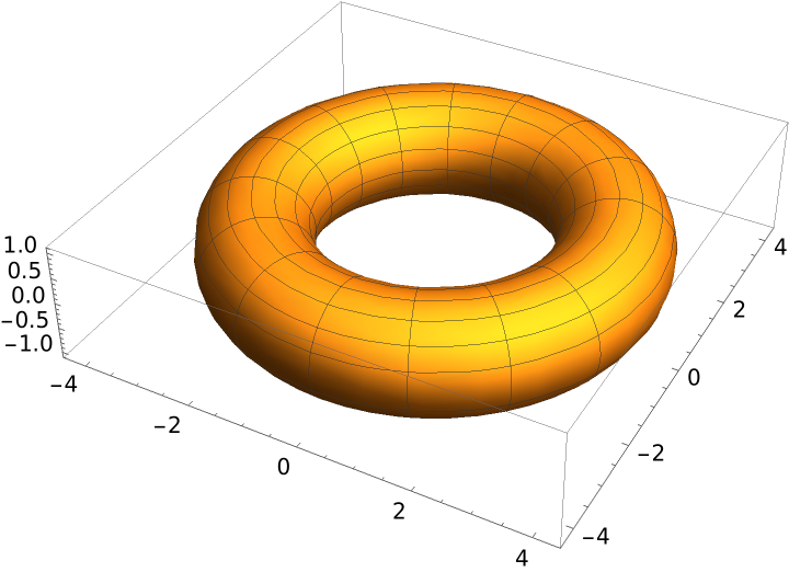 |
Transform tensors' different ranks regarding the local torus base with respect to transformation behavior. This is faster than transformation of an entire assembled rank-7 tensor):
| In[20]:= | ![(* Evaluate this cell to get the example input *) CloudGet["https://www.wolframcloud.com/obj/c5b72640-60b8-42a2-b25d-6392bd8b8098"]](https://www.wolframcloud.com/obj/resourcesystem/images/6d0/6d084720-3979-4be8-9075-48fe6c7d9d7f/65164ea645ec76e5.png) |
Local covariant base vector bi':
| In[21]:= |
Assemble the tensor term by contracting the right indices ci'j'k'l'sk'l'tj'bi≡ai'bi':
| In[22]:= |
| Out[22]= |
| In[23]:= |
| Out[23]= |
The result should be the same in the Cartesian system:
| In[24]:= |
| Out[24]= |
If the base vectors are not normalized ("Normalize"→False), i.e. if they have local-dependent lengths (and are not orthogonal in general reference systems either), the corresponding tensor components are transformed according to their co- and contravariant transformation behaviors. This leads to different representations of the same tensor object.
Here is an example of all four transforming possibilities of a rank-2 tensor to a local, non-normalized cylindrical system:
| In[25]:= | ![jacobianCylTransposed = Transpose@(CoordinateTransformData["Cylindrical" -> "Cartesian", "MappingJacobian", {r, \[Phi], z}]);](https://www.wolframcloud.com/obj/resourcesystem/images/6d0/6d084720-3979-4be8-9075-48fe6c7d9d7f/59b0a3dc9979834e.png) |
All coordinates transform the contravariant tij (default):
| In[26]:= | ![tConCon = ResourceFunction["TensorCoordinateTransform"][( {
{Subscript[\[Sigma], 11], Subscript[\[Sigma], 12], Subscript[\[Sigma], 13]},
{Subscript[\[Sigma], 21], Subscript[\[Sigma], 22], Subscript[\[Sigma], 23]},
{Subscript[\[Sigma], 31], Subscript[\[Sigma], 32], Subscript[\[Sigma], 33]}
} ), jacobianCylTransposed] // Simplify[#, r > 0] & // TraditionalForm](https://www.wolframcloud.com/obj/resourcesystem/images/6d0/6d084720-3979-4be8-9075-48fe6c7d9d7f/420f770fc403f182.png) |
| Out[26]= |  |
All coordinates transform the covariant tij:
| In[27]:= | ![tCovCov = ResourceFunction["TensorCoordinateTransform"][( {
{Subscript[\[Sigma], 11], Subscript[\[Sigma], 12], Subscript[\[Sigma], 13]},
{Subscript[\[Sigma], 21], Subscript[\[Sigma], 22], Subscript[\[Sigma], 23]},
{Subscript[\[Sigma], 31], Subscript[\[Sigma], 32], Subscript[\[Sigma], 33]}
} ), jacobianCylTransposed, "TransformationBehavior" -> "AllCovariant"] // Simplify[#, r > 0] & // TraditionalForm](https://www.wolframcloud.com/obj/resourcesystem/images/6d0/6d084720-3979-4be8-9075-48fe6c7d9d7f/5aaa344d3fd35bd6.png) |
| Out[27]= |  |
A tensor object with coordinates of mixed-transformation behavior tij:
| In[28]:= | ![tConCov = ResourceFunction["TensorCoordinateTransform"][( {
{Subscript[\[Sigma], 11], Subscript[\[Sigma], 12], Subscript[\[Sigma], 13]},
{Subscript[\[Sigma], 21], Subscript[\[Sigma], 22], Subscript[\[Sigma], 23]},
{Subscript[\[Sigma], 31], Subscript[\[Sigma], 32], Subscript[\[Sigma], 33]}
} ), jacobianCylTransposed, "TransformationBehavior" -> {"Cov", "Con"}] // Simplify[#, r > 0] & // TraditionalForm](https://www.wolframcloud.com/obj/resourcesystem/images/6d0/6d084720-3979-4be8-9075-48fe6c7d9d7f/1f9133a6b42fa4ca.png) |
| Out[28]= |  |
A tensor object with coordinates of opposite mixed-transformation behavior tji:
| In[29]:= | ![tCovCon = ResourceFunction["TensorCoordinateTransform"][( {
{Subscript[\[Sigma], 11], Subscript[\[Sigma], 12], Subscript[\[Sigma], 13]},
{Subscript[\[Sigma], 21], Subscript[\[Sigma], 22], Subscript[\[Sigma], 23]},
{Subscript[\[Sigma], 31], Subscript[\[Sigma], 32], Subscript[\[Sigma], 33]}
} ), jacobianCylTransposed, "TransformationBehavior" -> {"Con", "Cov"}] // Simplify[#, r > 0] & // TraditionalForm](https://www.wolframcloud.com/obj/resourcesystem/images/6d0/6d084720-3979-4be8-9075-48fe6c7d9d7f/2c804aa9dc9f5456.png) |
| Out[29]= |  |
Nomenclature referencing all indices together or each index separately is interchangeable:
| In[30]:= | ![(* Evaluate this cell to get the example input *) CloudGet["https://www.wolframcloud.com/obj/d0a5cd74-97e8-4a67-a3da-b8d6dadf7f50"]](https://www.wolframcloud.com/obj/resourcesystem/images/6d0/6d084720-3979-4be8-9075-48fe6c7d9d7f/06459425c6041332.png) |
| Out[30]= |
This is analogous for the covariant transformation:
| In[31]:= | ![(ResourceFunction["TensorCoordinateTransform"][( {
{Subscript[\[Sigma], 11], Subscript[\[Sigma], 12], Subscript[\[Sigma], 13]},
{Subscript[\[Sigma], 21], Subscript[\[Sigma], 22], Subscript[\[Sigma], 23]},
{Subscript[\[Sigma], 31], Subscript[\[Sigma], 32], Subscript[\[Sigma], 33]}
} ), jacobianCylTransposed, "TransformationBehavior" -> {"Cov", "Cov"}] == ResourceFunction["TensorCoordinateTransform"][( {
{Subscript[\[Sigma], 11], Subscript[\[Sigma], 12], Subscript[\[Sigma], 13]},
{Subscript[\[Sigma], 21], Subscript[\[Sigma], 22], Subscript[\[Sigma], 23]},
{Subscript[\[Sigma], 31], Subscript[\[Sigma], 32], Subscript[\[Sigma], 33]}
} ), jacobianCylTransposed, "TransformationBehavior" -> "AllCovariant"]) // Simplify[#, r > 0] &](https://www.wolframcloud.com/obj/resourcesystem/images/6d0/6d084720-3979-4be8-9075-48fe6c7d9d7f/09e4c34e5ca58892.png) |
| Out[31]= |
Transformed contravariant vector components with respect to normalized base vectors:
| In[32]:= | ![vNewConN = ResourceFunction["TensorCoordinateTransform"][vOld = {2, 8, 7}, mappingToNew = ( {
{2, 3, 1},
{1, 2, 2},
{1, 0, 1}
} ), "Normalize" -> True]](https://www.wolframcloud.com/obj/resourcesystem/images/6d0/6d084720-3979-4be8-9075-48fe6c7d9d7f/715dbd0929135edd.png) |
| Out[32]= |
The same transformed contravariant vector components with respect to non-normalized base vectors (default):
| In[33]:= |
| Out[33]= |
Transformed covariant normalized base vectors:
| In[34]:= | ![bNewCovN = ResourceFunction["TensorCoordinateTransform"][{e1, e2, e3}, mappingToNew, "TransformationBehavior" -> "AllCovariant", "Normalize" -> True] /. {e1 -> {1, 0, 0}, e2 -> {0, 1, 0}, e3 -> {0, 0, 1}}](https://www.wolframcloud.com/obj/resourcesystem/images/6d0/6d084720-3979-4be8-9075-48fe6c7d9d7f/13aaec0bf4ee665f.png) |
| Out[34]= |
The contraction of the assigned tensors should be produce invariance:
| In[35]:= |
| Out[35]= |
Tensor components with respect to an orthonormal cylindrical system:
| In[36]:= | ![tCylConCon = ResourceFunction["TensorCoordinateTransform"][( {
{Subscript[\[Sigma], 11], Subscript[\[Sigma], 12], Subscript[\[Sigma], 13]},
{Subscript[\[Sigma], 21], Subscript[\[Sigma], 22], Subscript[\[Sigma], 23]},
{Subscript[\[Sigma], 31], Subscript[\[Sigma], 32], Subscript[\[Sigma], 33]}
} ), Transpose@
CoordinateTransformData["Cylindrical" -> "Cartesian", "MappingJacobian", {r, \[Phi], z}], "Normalize" -> True] // Simplify[#, r > 0] &;
tCylConCon // TraditionalForm](https://www.wolframcloud.com/obj/resourcesystem/images/6d0/6d084720-3979-4be8-9075-48fe6c7d9d7f/4e3af97d7f8996bb.png) |
| Out[35]= |  |
TransformedField also assumes a normalized base:
| In[37]:= | ![TransformedField["Cartesian" -> "Cylindrical", ( {
{Subscript[\[Sigma], 11], Subscript[\[Sigma], 12], Subscript[\[Sigma], 13]},
{Subscript[\[Sigma], 21], Subscript[\[Sigma], 22], Subscript[\[Sigma], 23]},
{Subscript[\[Sigma], 31], Subscript[\[Sigma], 32], Subscript[\[Sigma], 33]}
} ), {x1, x2, x3} -> {r, \[Phi], z}] // Simplify // TraditionalForm](https://www.wolframcloud.com/obj/resourcesystem/images/6d0/6d084720-3979-4be8-9075-48fe6c7d9d7f/2907710e25b659ef.png) |
| Out[37]= |  |
| In[38]:= | ![(tCylConCon == TransformedField["Cartesian" -> "Cylindrical", ( {
{Subscript[\[Sigma], 11], Subscript[\[Sigma], 12], Subscript[\[Sigma], 13]},
{Subscript[\[Sigma], 21], Subscript[\[Sigma], 22], Subscript[\[Sigma], 23]},
{Subscript[\[Sigma], 31], Subscript[\[Sigma], 32], Subscript[\[Sigma], 33]}
} ), {x1, x2, x3} -> {r, \[Phi], z}]) // Simplify](https://www.wolframcloud.com/obj/resourcesystem/images/6d0/6d084720-3979-4be8-9075-48fe6c7d9d7f/1c8cb60247c393f8.png) |
| Out[38]= |
With orthonormal reference systems (e.g. normalized cylindrical systems), no distinction between co- and contravariant transformation behavior is required:
| In[39]:= | ![(tCylConCon ==
ResourceFunction["TensorCoordinateTransform"][( {
{Subscript[\[Sigma], 11], Subscript[\[Sigma], 12], Subscript[\[Sigma], 13]},
{Subscript[\[Sigma], 21], Subscript[\[Sigma], 22], Subscript[\[Sigma], 23]},
{Subscript[\[Sigma], 31], Subscript[\[Sigma], 32], Subscript[\[Sigma], 33]}
} ), Transpose@
CoordinateTransformData["Cylindrical" -> "Cartesian", "MappingJacobian", {r, \[Phi], z}], "TransformationBehavior" -> "AllCovariant", "Normalize" -> True]) // Simplify[#, r > 0] &](https://www.wolframcloud.com/obj/resourcesystem/images/6d0/6d084720-3979-4be8-9075-48fe6c7d9d7f/524720d2cc174e09.png) |
| Out[39]= |
| In[40]:= |
Hook's general law describes a linear relationship between the components of the rank-2 stress tensor σ and the two-stage strain tensor ε using the rank-4 tensor C: σij=Cijklεkl with the symmetries σij=σji, εkl=εlk and Eijkl=Ejikl=Eijlk=Eklij.
Components of the general, fully anisotropic stiffness tensor with initial symmetries:
| In[41]:= | ![cFull = Normal@
SymmetrizedArray[
pos_ :> Subscript[c, pos], {3, 3, 3, 3}, {{{2, 1, 3, 4}, 1}, {{1, 2, 4, 3}, 1}, {{3, 4, 1, 2}, 1}}];
cFull // MatrixForm](https://www.wolframcloud.com/obj/resourcesystem/images/6d0/6d084720-3979-4be8-9075-48fe6c7d9d7f/0ddd49f6a08e6206.png) |
| Out[37]= |  |
The number of independent components:
| In[42]:= |
| Out[42]= |
One plane of symmetry, rotated by 180 degrees, results in the same stiffness:
| In[43]:= |
| Out[44]= |
This results in a stiffness tensor with fewer independent components:
| In[45]:= | ![monoclinic = cFull /. (Flatten@(Solve[Thread@( Flatten@cFull == Flatten@ResourceFunction["TensorCoordinateTransform"][cFull,
rot3, "TransformationBehavior" -> "AllCovariant"])]));
monoclinic // MatrixForm](https://www.wolframcloud.com/obj/resourcesystem/images/6d0/6d084720-3979-4be8-9075-48fe6c7d9d7f/2dc1bb695efd66aa.png) |
| Out[20]= |  |
Determination and comparison of different material symmetries:
| In[46]:= | ![orthotrop = Fold[cFull /. (Solve[
Thread@(Flatten@cFull == Flatten@ResourceFunction[
"TensorCoordinateTransform"][#1, #2, "TransformationBehavior" -> "AllCovariant"])] // Flatten) &, cFull, {RotationMatrix[180 °, {0, 0, 1}], RotationMatrix[180 °, {0, 1, 0}]}];](https://www.wolframcloud.com/obj/resourcesystem/images/6d0/6d084720-3979-4be8-9075-48fe6c7d9d7f/5466b89466830cdf.png) |
| In[47]:= | ![transversalIso = Fold[cFull /. Quiet@ (* \[Alpha] only between 0° and 360° *)(Solve[
Thread@(Flatten@cFull == Flatten@ResourceFunction[
"TensorCoordinateTransform"][#1, #2, "TransformationBehavior" -> "AllCovariant"])] // Flatten) &, cFull, {RotationMatrix[180 °, {0, 0, 1}], RotationMatrix[180 °, {0, 1, 0}], RotationMatrix[\[Alpha], {1, 0, 0}]}];](https://www.wolframcloud.com/obj/resourcesystem/images/6d0/6d084720-3979-4be8-9075-48fe6c7d9d7f/7b827007a3b5e387.png) |
| In[48]:= | ![isotropic = Fold[cFull /. Quiet@(Solve[
Thread@(Flatten@cFull == Flatten@ResourceFunction[
"TensorCoordinateTransform"][#1, #2, "TransformationBehavior" -> "AllCovariant"])] // Flatten) &, cFull, {RotationMatrix[\[Alpha]1, {1, 0, 0}], RotationMatrix[\[Alpha]2, {0, 1, 0}], RotationMatrix[\[Alpha]3, {0, 0, 1}]}];](https://www.wolframcloud.com/obj/resourcesystem/images/6d0/6d084720-3979-4be8-9075-48fe6c7d9d7f/194cbecf3724f5c5.png) |
Summary:
| In[49]:= | ![(<|"Material behaviour" -> #2, "Stiffness Tensor" -> (#1 // MatrixForm), "Independent Components" -> (Cases[#1, _Subscript, \[Infinity]] //
Union), "Number of independent components" -> Length[Cases[#1, _Subscript, \[Infinity]] // Union], "Description" -> #3|>) & @@@ {{monoclinic, "Monoclinic", "One symmetric plane"},
{orthotrop, "Orthotropic", "Two (three) symmetric planes"},
{transversalIso, "Transversal isotropic", "Two symmetric planes transversal isometric"},
{isotropic, "Isotropic", "All planes isometric"}} // Dataset](https://www.wolframcloud.com/obj/resourcesystem/images/6d0/6d084720-3979-4be8-9075-48fe6c7d9d7f/03817e84e4032879.png) |
| Out[49]= | 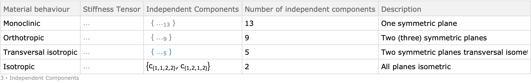 |
This work is licensed under a Creative Commons Attribution 4.0 International License