Function Repository Resource:

StratonovichProcessChangeVariables

Source Notebook

Perform a change of state variables for a Stratonovich stochastic process

Contributed by: Bruno Tenorio

ResourceFunction["StratonovichProcessChangeVariables"][straProc, u, trans]

changes the state variable of the Stratonovich process straProc to u using the transformation trans.

ResourceFunction["StratonovichProcessChangeVariables"][straProc,{u1,u2,},trans]

changes the state variables of the Stratonovich process to {u1,u2,}.

Details and Options

ResourceFunction["StratonovichProcessChangeVariables"] performs a change of state variables for a StratonovichProcess, including the transformation of initial conditions, and returns a new StratonovichProcess.
The drift a and diffusion (noise) b of the input process can follow any of the specifications allowed by StratonovichProcess.
The new diffusion (noise) term b' is calculated via the Jacobian matrix J of the corresponding mapping as b' = J.b.
Because Stratonovich processes obey standard calculus, the new drift term a' is calculated using the chain rule. For each component fi of the transformation: (a')i = ∂fi/∂t+∇fi . a, the derivative with respect to time variable includes transformations that have explicit time dependence.
The transformation trans can have the forms:
Assumptions can be supplied to specify restrictions on the state variables and parameters. They are used for inverse mapping, solving and expression simplification.
Please see the documentation page for StratonovichProcess for additional details on variables and their meaning.

Examples

Basic Examples (6) 

Define a Stratonovich process:

In[1]:=
procX = StratonovichProcess[{0, 1}, {x, x0}, t]
Out[1]=

Square transformation of the process:

In[2]:=
ResourceFunction["StratonovichProcessChangeVariables"][procX, y, y == x^2]
Out[2]=

Start with a Stratonovich process:

In[3]:=
proc = StratonovichProcess[{0, 1}, {x, x0}, t]
Out[3]=

Cubic transformation of a process:

In[4]:=
ResourceFunction["StratonovichProcessChangeVariables"][proc, y, y == x^3]
Out[4]=

Start with a geometric Brownian motion process:

In[5]:=
gbm = StratonovichProcess@
  GeometricBrownianMotionProcess[\[Mu], \[Sigma], x0]
Out[5]=

Log transformation of the process:

In[6]:=
transformed = ResourceFunction["StratonovichProcessChangeVariables"][gbm, y, y == Log[\[FormalX]]]
Out[6]=

Show the PDF of the transformed process:

In[7]:=
Simplify[(PDF@transformed[t])[x]]
Out[7]=

Start with an Ornstein-Uhlenbeck process:

In[8]:=
ou = StratonovichProcess@
  OrnsteinUhlenbeckProcess[\[Mu], \[Sigma], \[Theta], x0]
Out[8]=

Log transformation of the process:

In[9]:=
ResourceFunction["StratonovichProcessChangeVariables"][ou, y, y == Log[\[FormalX]]]
Out[9]=

Define the following Stratonovich process:

In[10]:=
proc = StratonovichProcess[{1, {\[Sigma] x}}, {x, x0}, t]
Out[10]=

Perform a reciprocal transformation:

In[11]:=
ResourceFunction["StratonovichProcessChangeVariables"][proc, y, y == 1/x]
Out[11]=

Start with a 2D process:

In[12]:=
proc = StratonovichProcess[{{0, 0}, IdentityMatrix[2]}, {x, y}, t]
Out[12]=

Two variable linear transformation of the process:

In[13]:=
ResourceFunction[
 "StratonovichProcessChangeVariables"][proc, {u, v}, {u == x + y, v == x - y}]
Out[13]=

Scope (4) 

Start with an OrnsteinUhlenbeck process:

In[14]:=
ou = StratonovichProcess@
  OrnsteinUhlenbeckProcess[\[Mu], \[Sigma], \[Theta], x0]
Out[14]=

Consider the transformation y =θ t(x-μ) that is time dependent:

In[15]:=
transformed = ResourceFunction["StratonovichProcessChangeVariables"][ou, y, y == E^(\[Theta] \[FormalT]) (\[FormalX] - \[Mu])];

Check the process is drift-less for this transformation:

In[16]:=
transformed["Drift"] == {0}
Out[16]=

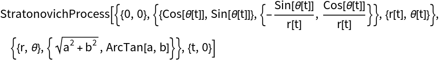
Define a 2D Stratonovich process:

In[17]:=
sp2D = StratonovichProcess[{{0, 0}, IdentityMatrix[2]}, {{x, y}, {a, b}}, t]
Out[17]=

Transform coordinates to polar:

In[18]:=
ResourceFunction[
 "StratonovichProcessChangeVariables"][sp2D, {r, \[Theta]}, "Cartesian" -> "Polar"]
Out[18]=

Start with a general process with drift a and diffusion b:

In[19]:=
spLinear = StratonovichProcess[{a, b}, {x, x0}, {t, t0}]
Out[19]=

Time dependent scaling:

In[20]:=
resTimeDep = ResourceFunction["StratonovichProcessChangeVariables"][
  spLinear, {y}, {y == x/t}]
Out[20]=

Define a process in cylindrical coordinates:

In[21]:=
proc3D = StratonovichProcess[{{1/\[Rho], 0, 0}, {\[Sigma]/(\[Rho]^2 + z^2), 0, \[Sigma] z}}, {{\[Rho], \[Phi],
     z}, {\[Rho]0, \[Phi]0, z0}}, t]
Out[21]=

Perform a transformation to spherical coordinates using long names notation:
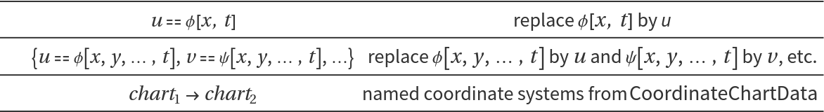
In[22]:=
ResourceFunction[
 "StratonovichProcessChangeVariables"][proc3D, {r, \[FormalTheta], \[CurlyPhi]}, {"Cylindrical", "Euclidean", 3} -> {"Spherical", "Euclidean", 3}]
Out[22]=

Options (3) 

Assumptions (3) 

Start with a Stratonovich process:

In[23]:=
procX = StratonovichProcess[{0, 1}, {x, 0}, t];

Tangent/Cauchy transformation of Stratonovich process:

In[24]:=
ResourceFunction["StratonovichProcessChangeVariables"][procX, y, y == Tan[x]]
Out[24]=

Specify a solving branch for 0<=x<2π:

In[25]:=
procY = ResourceFunction["StratonovichProcessChangeVariables"][procX, y, y == Tan[x], Assumptions -> {0 <= x < 2 \[Pi]}]
Out[25]=

Stratonovich process generated from a CoxIngersollRoss process:

In[26]:=
proc = StratonovichProcess@
  CoxIngersollRossProcess[\[Theta], \[Sigma], \[Kappa], x0]
Out[26]=

Square root(Lamperti) transformation:

In[27]:=
ResourceFunction[
 "StratonovichProcessChangeVariables"][proc, y, {y == Sqrt[\[FormalX]]},
  Assumptions -> {y > 0, \[FormalX] > 0}]
Out[27]=

Define the following process:

In[28]:=
proc = StratonovichProcess[{\[Mu], \[Sigma]}, {x, x0}, t]
Out[28]=

Transform the process, pass the transformation in implicit form x = Log(y/1-y):

In[29]:=
ResourceFunction["StratonovichProcessChangeVariables"][proc, y, x == Log[y/(1 - y)]]
Out[29]=

Applications (15) 

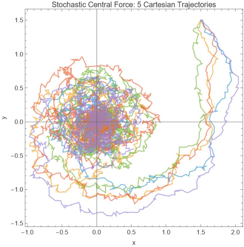
2D stochastic trapping central force (5) 

Define a stochastic process representing harmonic oscillator trap(including a magnetic effect) in Cartesian coordinates:

In[30]:=
spMagnetic = StratonovichProcess[{{-\[Gamma] x + B y, -\[Gamma] y - B x}, {{\[Sigma], 0}, {0, \[Sigma]}}}, {{x, y}, {x0, y0}}, t]
Out[30]=

Change to polar coordinates that are more suitable to the problem:

In[31]:=
spPolar = ResourceFunction["StratonovichProcessChangeVariables"][
  spMagnetic, {r, \[Phi]}, "Cartesian" -> "Polar"]
Out[31]=

Set up parameters and simulate 5 paths:

In[32]:=
paths = RandomFunction[
   spPolar /. {\[Gamma] -> 0.5, B -> 2, \[Sigma] -> 0.3, x0 -> 1.5, y0 -> 1.5}, {0, 20, 0.01}, 5];

Swap back to Cartesian coordinates for plotting:

In[33]:=
cartesianPaths = Table[Map[{#[[2, 1]] Cos[#[[2, 2]]], #[[2, 1]] Sin[#[[2, 2]]]} &, p], {p, paths["Paths"]}];

Plot the paths:

In[34]:=
ListLinePlot[cartesianPaths, Sequence[
 AspectRatio -> 1, PlotStyle -> Directive[
Thickness[0.004], 
Opacity[0.7]], PlotLabel -> "Stochastic Central Force: 5 Cartesian Trajectories", Frame -> True, FrameLabel -> {"x", "y"}, PlotRange -> All]]
Out[34]=

Gompertz stochastic growth (4) 

Define a stochastic process representing the Gompertz growth equation with noise:

In[35]:=
proc = StratonovichProcess[{\[FormalCapitalN] (a - b Log[\[FormalCapitalN]]), \[Sigma] \[FormalCapitalN]}, {\[FormalCapitalN], N0}, t]
Out[35]=

Logarithmic variable change:

In[36]:=
transformed = ResourceFunction["StratonovichProcessChangeVariables"][proc, X, X == Log[\[FormalCapitalN]], Assumptions -> {X > 0, N0 > 1}];

The process becomes OrnsteinUhlenbeck after the transformation with parameters:

In[37]:=
ou = StratonovichProcess@
   OrnsteinUhlenbeckProcess[a/b, \[Sigma], b, Log[N0]];

Check the PDF are the same:

In[38]:=
SameQ @@ Comap[(PDF@*#) & /@ {transformed, ou}, t]
Out[38]=

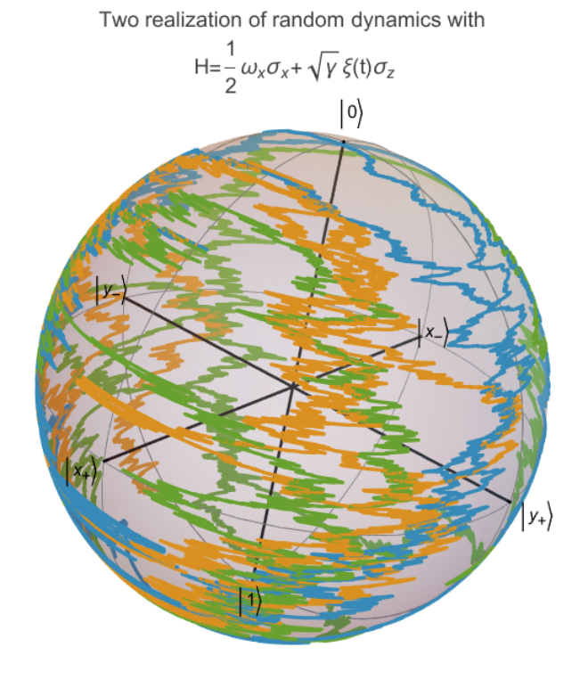
Stochastic Schrodinger equation (6) 

Define the terms with ⅆt and ∘ⅆWt of the stochastic differential equation in Cartesian coordinates, the terms originate from the following equation 
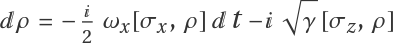
∘ⅆWt for some density matrix ρ expressed as a Bloch vector:

In[39]:=
SDEnonRandom = {0, -z \[Omega]x, y \[Omega]x};
SDErandom = {-2 y Sqrt[\[Gamma]], 2 x Sqrt[\[Gamma]], 0};

Build the Stratonovich process:

In[40]:=
procCartesian = StratonovichProcess[{SDEnonRandom, SDErandom}, {{x, y, z}, {x0, y0, z0}}, t]
Out[40]=

Transform to spherical coordinates:

In[41]:=
procSpherical[{\[Omega]x_, \[Gamma]_}, {x0_, y0_, z0_}] = ResourceFunction["StratonovichProcessChangeVariables"][
  procCartesian, {r, \[Theta], \[Phi]}, "Cartesian" -> "Spherical"]
Out[41]=

Generate 100 realizations for the density matrix:

In[42]:=
paths = RandomFunction[
   procSpherical[{2, .2}, {1/Sqrt[2], 0, 1/Sqrt[2]}], {0, 10, 0.001}, 100];

Switch back to Cartesian coordinates for plotting:

In[43]:=
cartesianBlochPaths = TimeSeriesMap[{#[[1]] Sin[#[[2]]] Cos[#[[3]]], #[[
       1]] Sin[#[[2]]] Sin[#[[3]]], #[[1]] Cos[#[[2]]]} &, paths];

Show the Bloch vector trajectories on the Bloch sphere for three realizations:

In[44]:=
Show[ResourceFunction[
ResourceObject[<|"Name" -> "BlochSpherePlot", "ShortName" -> "BlochSpherePlot", "UUID" -> "fcb3b840-6ae5-4883-a256-1573cc958ffc", "ResourceType" -> "Function", "Version" -> "1.0.0", "Description" -> "Plot the Bloch sphere", "RepositoryLocation" -> URL[
      "https://www.wolframcloud.com/obj/resourcesystem/api/1.0"], "SymbolName" -> "FunctionRepository`$260e867144764f229d14c35cdf9d34d9`BlochSpherePlot", "FunctionLocation" -> CloudObject[
      "https://www.wolframcloud.com/obj/858bce1b-d11f-4b5c-8673-c3107cef60fb"]|>, ResourceSystemBase -> Automatic]][], ListLinePlot3D[cartesianBlochPaths["ValueList"][[;; 3]]], PlotLabel -> "Two realization of random dynamics with\n H=\!\(\*FractionBox[\(1\), \(2\)]\)\!\(\*SubscriptBox[\(\[Omega]\), \(x\)]\)\!\(\*SubscriptBox[\(\[Sigma]\), \(x\)]\)+\!\(\*SqrtBox[\(\[Gamma]\)]\)\[Xi](t)\!\(\*SubscriptBox[\(\[Sigma]\), \(z\)]\)"]
Out[44]=

Publisher

Mads Bahrami

Requirements

Wolfram Language 13.3 (June 2023) or above

Version History

  • 1.0.0 – 14 January 2026

Related Resources

License Information