Wolfram Function Repository
Instant-use add-on functions for the Wolfram Language
Function Repository Resource:
Move back and forth from the squared space or square root space of an algebraic number field
ResourceFunction["SqrtSpace"][root,pts] while tracking signs, converts Cartesian pts2 to algebraic values in |
Using ϕ, GoldenRatio or Fibonacci’s rabbit constant, convert points to the algebraic number field ![]() and build the Fermat triangle:
and build the Fermat triangle:
| In[1]:= | ![\[Phi] = GoldenRatio;
points = {{0, 0}, {0, 1}, {-Sqrt[\[Phi]], 0}};
Column[{ResourceFunction["SqrtSpace"][\[Phi], points], Graphics[{EdgeForm[Black], Yellow, Polygon[points]}]}]](https://www.wolframcloud.com/obj/resourcesystem/images/aa9/aa9b4e6b-9bdf-4b2e-bfd2-7cd4f337f73e/5bad36f088ff0af1.png) |
| Out[3]= | 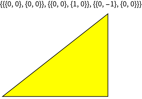 |
Using ψ, the supergolden ratio or Narayana’s cow constant, convert points to the algebraic number field ![]() and build the supergolden triangle:
and build the supergolden triangle:
| In[4]:= | ![\[Psi] = Root[-1 - #1^2 + #1^3 &, 1];
points = {{0, 0}, {1/2, Sqrt[3]/2}, {-\[Psi], 0}};
Column[{ResourceFunction["SqrtSpace"][\[Psi], points], Graphics[{EdgeForm[Black], Yellow, Polygon[points]}]}]](https://www.wolframcloud.com/obj/resourcesystem/images/aa9/aa9b4e6b-9bdf-4b2e-bfd2-7cd4f337f73e/07ac5b2a9257a75a.png) |
| Out[6]= |  |
Convert back to the original points:
| In[7]:= |
| Out[7]= |
Under "Neat Examples" in GeometricScene, there is a mysterious output after "Decompose a triangle into similar triangles":
| In[8]:= | ![RandomInstance[GeometricScene[{a, b, c, d, g, e, f}, {
p0 == Polygon[{e, g, f}],
p1 == Style[Polygon[{a, b, c}], Cyan],
p2 == Style[Polygon[{b, c, d}], Purple],
p3 == Style[Polygon[{d, c, g}], Red],
p4 == Style[Polygon[{g, c, a}], Green],
p5 == Style[Polygon[{e, d, b}], Blue],
p6 == Style[Polygon[{g, a, f}], Magenta],
GeometricAssertion[{p0, p1, p2, p3, p4, p5, p6}, "Similar"],
a == {-1/2, 0}, b == {1/2, 0}}], RandomSeeding -> 5]](https://www.wolframcloud.com/obj/resourcesystem/images/aa9/aa9b4e6b-9bdf-4b2e-bfd2-7cd4f337f73e/1ccb570687f5ab09.png) |
| Out[8]= | 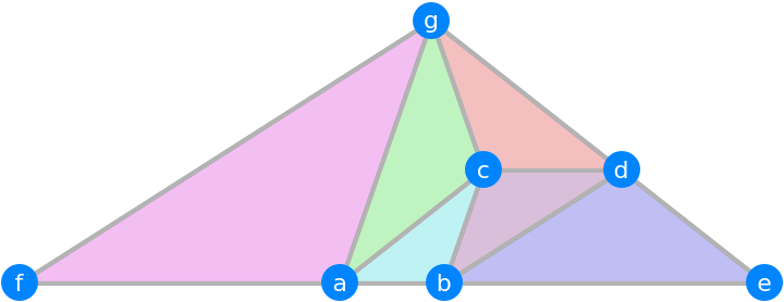 |
This triangle is in the algebraic number field / geometric space of ![]() where ρ is the plastic constant:
where ρ is the plastic constant:
| In[9]:= | ![\[Rho] = Root[-1 - #1 + #1^3 &, 1]; vals = {{{-(1/4), 0, 0}, {0, 0, 0}}, {{1/4, 0, 0}, {0, 0, 0}}, {{0, 1/4, 1/4}, {-(1/4), 3/4, 1/4}}, {{1, 5/4, 5/4}, {-(1/4),
3/4, 1/4}}, {{9/4, 4, 3}, {0, 0, 0}}, {{-(9/4), -4, -3}, {0, 0, 0}}, {{1/4, 1/4, -(1/4)}, {1, 7/4, 7/4}}}; triangles = {{1, 2, 3}, {2, 3, 4}, {4, 3, 7}, {7, 3, 1}, {5, 4, 2}, {7, 1, 6}};
points = ResourceFunction["SqrtSpace"][\[Rho], vals];
Graphics[{EdgeForm[
Black], {Hue[Area[#]], #} & /@ (Polygon[points[[#]]] & /@ triangles)}]](https://www.wolframcloud.com/obj/resourcesystem/images/aa9/aa9b4e6b-9bdf-4b2e-bfd2-7cd4f337f73e/0570214f703c4cf8.png) |
| Out[11]= | 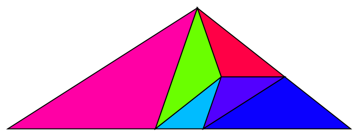 |
Convert the points back to original values:
| In[12]:= |
| Out[12]= |  |
A simple application of ToNumberField does not recognize the points as being in either ![]() or
or ![]() , but does recognize the values when they get squared:
, but does recognize the values when they get squared:
| In[13]:= | ![\[Rho] = Root[-1 - #1 + #1^3 &, 1];
Column[{
Quiet@ToNumberField[points[[3]], \[Rho]],
Quiet@ToNumberField[points[[3]], Sqrt[\[Rho]]],
ToNumberField[points[[3]]^2, \[Rho]]}]](https://www.wolframcloud.com/obj/resourcesystem/images/aa9/aa9b4e6b-9bdf-4b2e-bfd2-7cd4f337f73e/6ee51faaea2232e4.png) |
| Out[14]= | 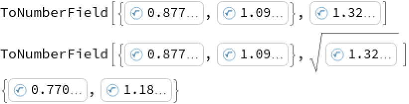 |
These values are algebraic numbers:
| In[15]:= |
| Out[15]= |
The actual point is also a pair of algebraic numbers:
| In[16]:= |
| Out[16]= |
The signs here happen to be positive, so taking the square root of the algebraic version does not require extra steps:
| In[17]:= |
| Out[17]= |
Convert 19 points from the algebraic number field ![]() of the plastic constant ρ into 3D coordinates:
of the plastic constant ρ into 3D coordinates:
| In[18]:= | ![\[Rho] = Root[-1 - #1 + #1^3 &, 1];
points = ResourceFunction[
"SqrtSpace"][\[Rho], {{{-19, 0, 19}, {19, 76, 57}, {0, 0, 0}}, {{-76, -57, 57}, {0, 19, 57}, {0, 0, 0}}, {{0, -19, 0}, {76, 133, 76},
{0, 0, 0}}, {{76, 76, 0}, {0, 0, 0}, {0, 0, 0}}, {{76, 95, 76}, {76, 133, 76}, {0, 0, 0}}, {{-38, 0, 19}, {38, 0, 19}, {0, 0, 0}}, {{95, 19, -57}, {-19, 57, -19}, {0, 0, 0}}, {{0, -19, 19}, {0, 19, 57}, {0, 0, 0}}, {{-38, 0, 19}, {42, 68, 43}, {-4, 8, 52}}, {{19, 38, -38}, {17, 42, 26}, {40, -4, 12}}, {{19, 38, -38}, {9, -18, 54}, {-28, 56, -16}}, {{0, -19, 19}, {36, 99,
45}, {40, -4, 12}}, {{-152, -171, -76}, {76, 133, 76}, {0, 0, 0}}, {{76, 95, -76}, {76, 133, 76}, {0, 0, 0}}, {{76, -57, 0}, {76, 133, 76}, {0, 0, 0}}, {{76, 76, 0}, {16, 44, 20}, {60, 108, 56}}, {{95, 19, -57}, {49, 73, 9}, {8, 60, 48}}, {{-76, -57, 57}, {36, 99, 45}, {40, -4, 12}}, {{-19, 0, 19}, {47, 96, 73}, {-28, 56, -16}}}/76]](https://www.wolframcloud.com/obj/resourcesystem/images/aa9/aa9b4e6b-9bdf-4b2e-bfd2-7cd4f337f73e/11ebe9601fe8ef85.png) |
| Out[19]= | 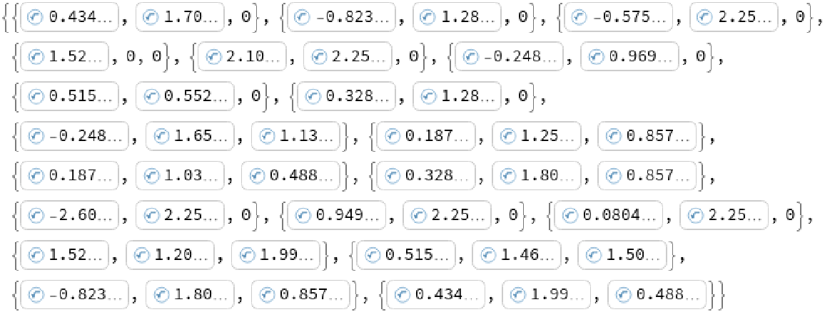 |
Find the distances between these points in terms of powers of ![]() :
:
| In[20]:= |
| Out[20]= |  |
Plot out the points:
| In[21]:= | ![Graphics3D[{Map[Function[x, Tube[points[[x]], .02]], Subsets[Range[19], {2}]], Table[Sphere[points[[n]], .07], {n, 1, 19}]}, Boxed -> False,
ImageSize -> Large, ViewPoint -> {0, 1, 40}]](https://www.wolframcloud.com/obj/resourcesystem/images/aa9/aa9b4e6b-9bdf-4b2e-bfd2-7cd4f337f73e/7e3ecfd2ebd7a6a3.png) |
| Out[21]= | 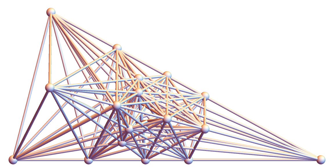 |
Wolfram Language 11.3 (March 2018) or above
This work is licensed under a Creative Commons Attribution 4.0 International License