Basic Examples (5)
Plot a spirograph:
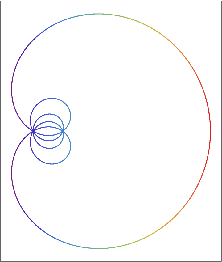
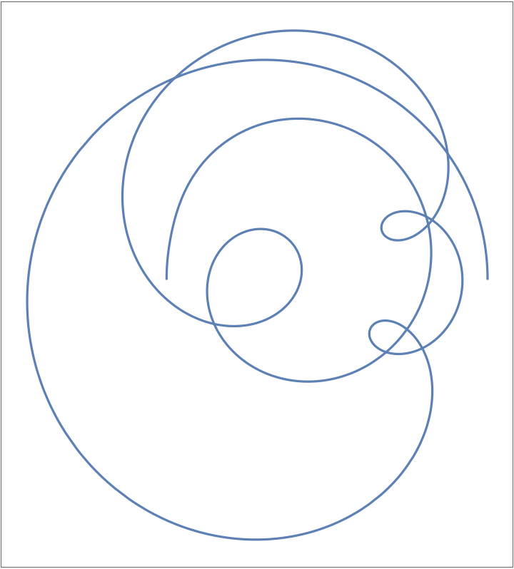
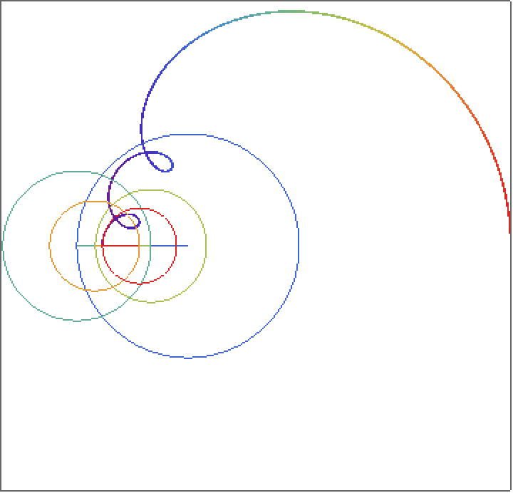
A more complicated spirograph:
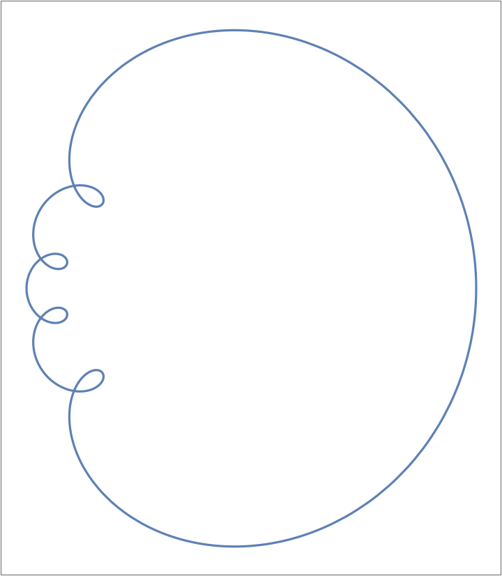
Half of the path of the spirograph:
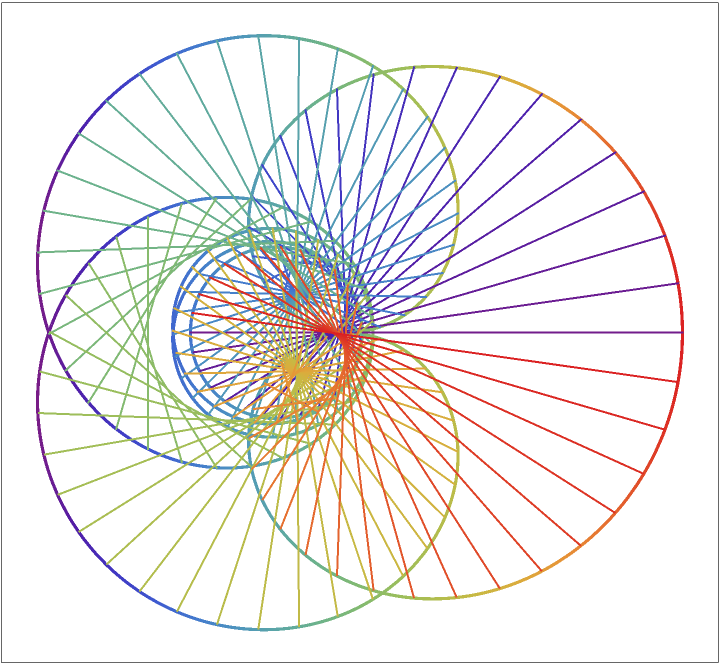
Convert the curve to a polygon:
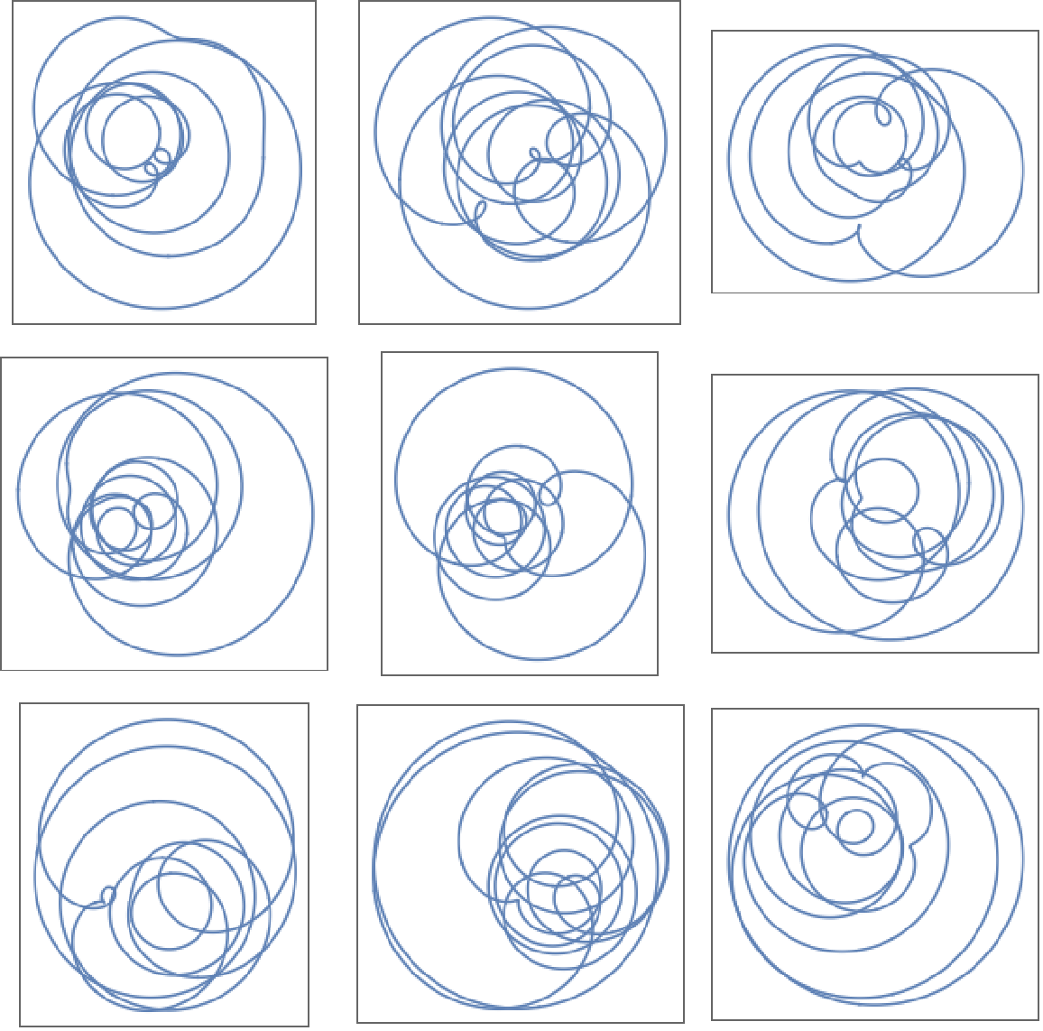
Spirographs with random values:
Applications (7)
Spirographs had an important application in the 1940s, when they were used for the "manual" solution of polynomial equations of higher degree. To understand this, consider the following polynomial poly in the variable z:
Replace the variable z by its polar form, r ⅇⅈ φ, where r and φ are the absolute value and phase or argument of z:
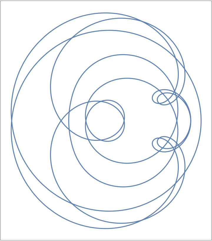
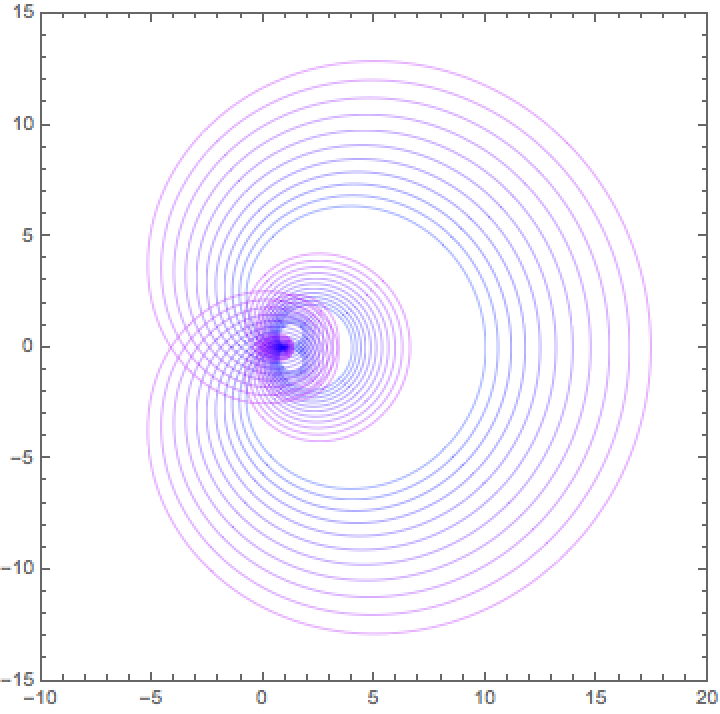
Show the spirographs for a range of values of r:
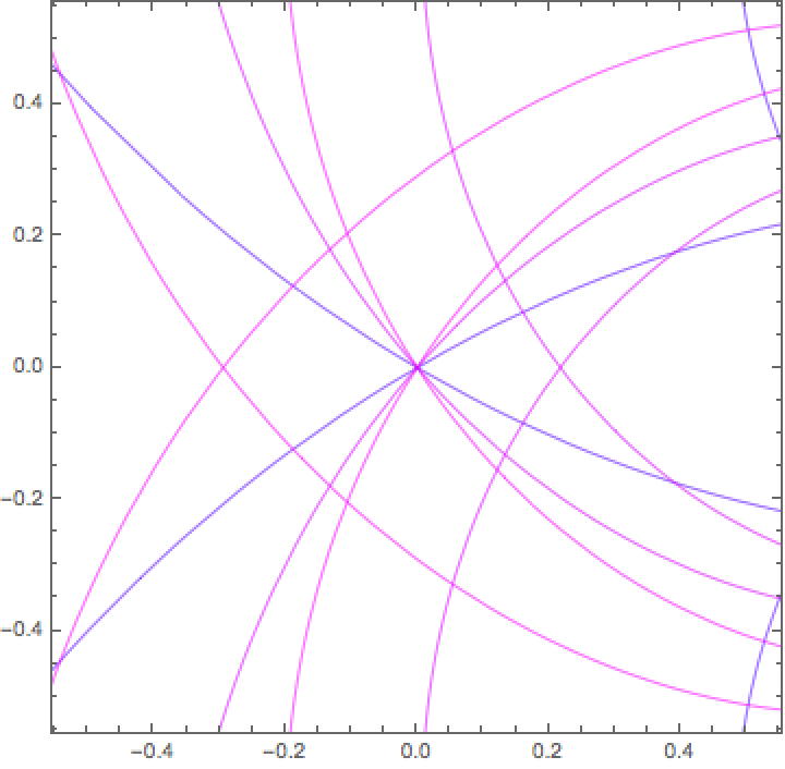
Zoom to a neighborhood of the origin:
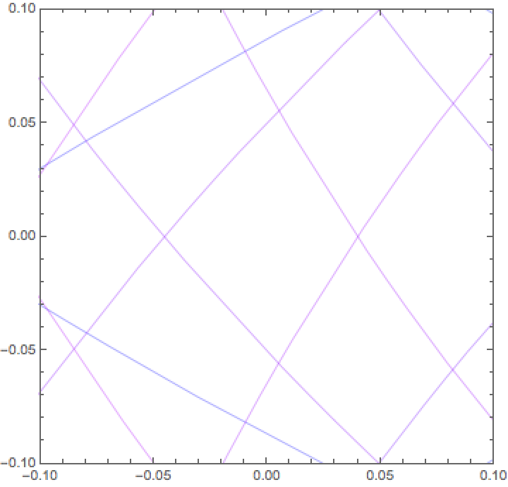
Here is an even closer look:
These are absolute values and arguments of the zeros of the polynomial:
The spirograph curves corresponding to these absolute values all go through the origin:
An analog circuit was used to vary r and the corresponding spirographs were monitored using an oscilloscope. Further analysis to determine φ led to approximations of the zeros of the polynomial.

![ResourceFunction["Spirograph"][\!\(
\*UnderoverscriptBox[\(\[Sum]\), \(j = 1\), \(7\)]\(\((
\*FractionBox[\(j\), \(6\)] + Sin[j])\)\
\*SuperscriptBox[\(E\), \(j\ I\ \ \[CurlyPhi]\)]\)\), \[CurlyPhi], "MaurerPolygons" -> {100, 200}, ColorFunction -> "Rainbow"]](https://www.wolframcloud.com/obj/resourcesystem/images/9ff/9ff65e59-cbc6-44e7-bba3-1f3b99f83af6/77a8d16e03d4935d.png)
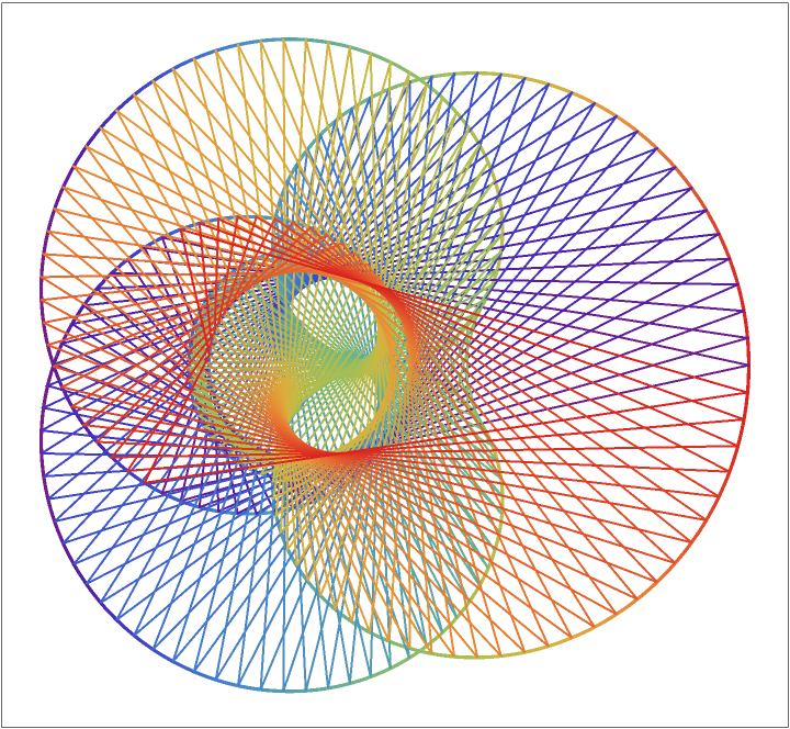
![ResourceFunction["Spirograph"][\!\(
\*UnderoverscriptBox[\(\[Sum]\), \(j = 1\), \(5\)]
\*FractionBox[
SuperscriptBox[\(E\), \(j\ I\ \[CurlyPhi]\)], \(j + 1\)]\), \[CurlyPhi], \[Pi], "ShowCircles" -> True, ColorFunction -> "Rainbow", PlotRange -> {{-0.84, 1.45}, {-1.1, 1.1}}]](https://www.wolframcloud.com/obj/resourcesystem/images/9ff/9ff65e59-cbc6-44e7-bba3-1f3b99f83af6/5a57ee3a92e21dde.png)
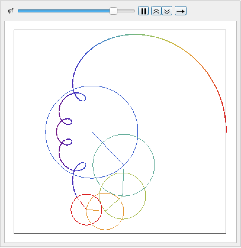
![Animate[ResourceFunction["Spirograph"][\!\(
\*UnderoverscriptBox[\(\[Sum]\), \(j = 1\), \(5\)]
\*FractionBox[
SuperscriptBox[\(E\), \(j\ I\ \[CurlyPhi]\)], \(j + 1\)]\), \[CurlyPhi], \[CurlyPhi]f, "ShowCircles" -> True, ColorFunction -> "Rainbow", PlotRange -> {{-0.84, 1.45}, {-1.1, 1.1}}], {\[CurlyPhi]f, 0.1, 2 \[Pi]}]](https://www.wolframcloud.com/obj/resourcesystem/images/9ff/9ff65e59-cbc6-44e7-bba3-1f3b99f83af6/720996022228da72.png)
![Show[Table[
ResourceFunction["Spirograph"][poly1, \[CurlyPhi], PlotStyle -> {Thickness[0.001], Hue[0.71 (r - 0.1)]}, FrameTicks -> True, PlotRange -> {{-10, 20}, {-15, 15}}], {r, 1.0, 1.2, 0.02}]]](https://www.wolframcloud.com/obj/resourcesystem/images/9ff/9ff65e59-cbc6-44e7-bba3-1f3b99f83af6/7a83943d15c50759.png)
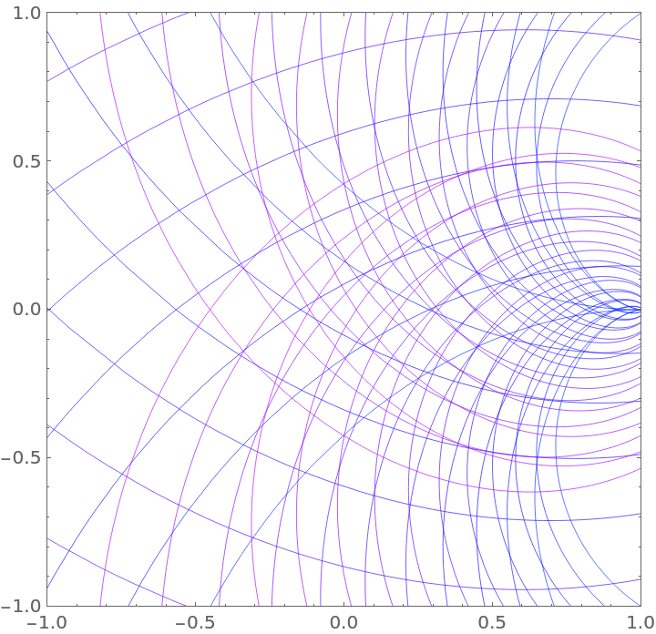
![Show[ResourceFunction["Spirograph"][poly1 /. r -> #, \[CurlyPhi], PlotStyle -> {Thickness[0.001], Hue[0.7 #1]}] & /@ First /@ %, FrameTicks -> True, PlotRange -> {{-(1/2), 1/2}, {-(1/2), 1/2}}]](https://www.wolframcloud.com/obj/resourcesystem/images/9ff/9ff65e59-cbc6-44e7-bba3-1f3b99f83af6/5512b1e9618ecbb5.png)