Details and Options
ResourceFunction["SchmidtArrangements"] takes the following options:
| "Color" | Black | the specification of a color or color palette |
| "Circle" | True | specify if circles or disks are used for the picture |
| "Transparency" | 0.0 | specify the transparency value or transparency mode |
| "Filter" | Circle[{0,0.5},Sqrt[0.25]] | specify the shape used to clip the picture |
| "MinCurvature" | 0 | specify the minimum circle curvature in the picture |
| "MaxCurvature" | 20 | specify the maximum circle curvature in the picture |
| "XMax" | 1.0 | maximum horizontal coordinate value used to search for new circles |
| "YMax" | 1.0 | maximum vertical coordinate value used to search for new circles |
| "Containment" | True | specify if a circle can contain other circles |
| "Precompute" | False | specify if the pre-computation mode is enabled |
"Color" can be used to specify a color like
Black.
"Color" can be a color palette: "Color"
→ColorData["SolarColors"].
In a Schmidt arrangement, all curvatures are an integer multiple of a common value. So, curvatures are expressed as integers. The value for the color palette is normalized between 0.0 and 1.0 such that 0.0 corresponds to the minimum integer curvature and 1.0 to the maximum.
"Color" can be a special color palette provided with the ResourceFunction["SchmidtArrangements"] function: "Color"→{"ColorPool",{1,0}}.
Special palettes are defined with {"nameofpalette",{a,b}} or {"nameofpalette",{n,a,b}}.
The color index is given by (c*a+b) mod n where c is the curvature expressed as an integer.
n can be any number less than or equal to the number of colors in a given palette.
The "Color" option can also be a special gradient which is an interpolation between palettes as follows: "Color"→{"Gradient",{colfuncstart,colfuncend}}.
The value of the "Color" option can either be a
ColorData expression or a special color palette.
The special color palettes recognized by this function are:
| Length of the palette | Color names |
| 4 colors | "ColorCu", "ColorSaul", "ColorAntique", "ColorGreen", "Color92", "ColorGolden", "ColorPool", "ColorDistinct", "ColorNightlife", "ColorA", "ColorB", "ColorC" |
| 5 colors | "Color5" |
| 6 colors | "Color6", "Color6Alt", "Color6Seeds" |
| 24 colors | "Color24" |
These names come from the original Sage notebook by Katherine E. Stange and Daniel E. Martin.
Use the setting "Circle"
→ False to get disks rather than circles in the diagram.
"Transparency" is used to vary the transparency according to the circle curvature. Two settings are supported: "Increasing" and "Decreasing".
"Filter" is used to clip the final picture with a
Rectangle or
Circle. By default, a circle is used for clipping. Note that this setting will only check the center of the circles and draw circles if their center is inside the shape. The circle boundary can be outside the clipping shape.
"MinCurvature" and "MaxCurvature" limit the curvatures. These are the only two options which are used both in precompute and drawing mode. They can have different values for each mode.
"XMax" and "YMax" are used to limit the region of the plane where circles are searched.
"Containment" is set to
True when a circle cannot contain any other circles. Circles contained in another circle will be removed.
"Precompute" is used to separate the compute phase from the styling and drawing phase.

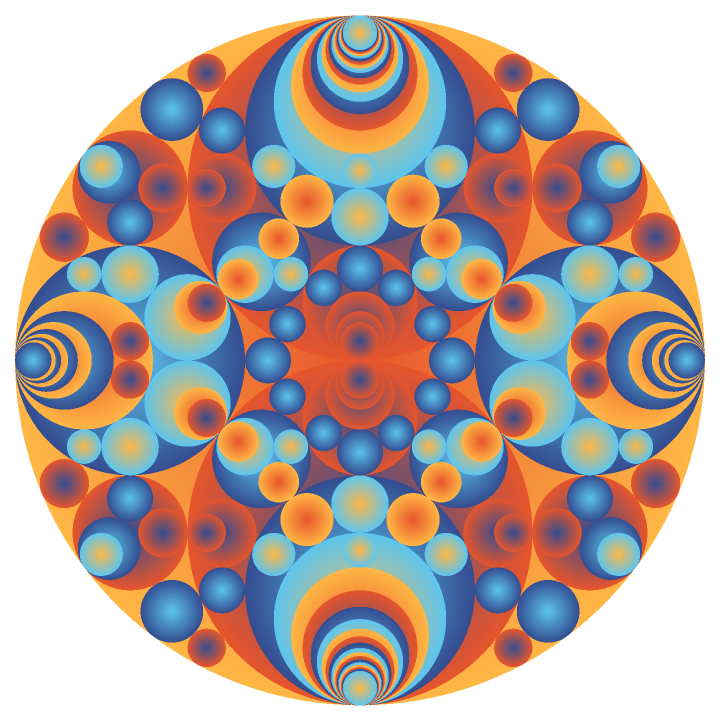
![ResourceFunction["SchmidtArrangements"][-1, "MaxCurvature" -> 40, "Color" -> {"ColorSaul", {2, 1, 1}},
"Transparency" -> "Increasing", "Filter" -> Rectangle[{-0.1, -0.1}, {1.1, 1.1}],
PlotRange -> {{0, 1}, {0, 1}}]](https://www.wolframcloud.com/obj/resourcesystem/images/330/33072f77-33e8-4cd6-9838-8fe0b21d493e/78e3e39c5edc4d49.png)

![ResourceFunction["SchmidtArrangements"][-2, "MaxCurvature" -> 40, "Color" -> {"ColorSaul", {2, 1, 1}},
"Transparency" -> "Increasing", "Filter" -> Rectangle[{-0.1, -0.1}, {1.1, Sqrt[2.0] + 0.1}],
PlotRange -> {{0, 1}, {0, Sqrt[2.0]}}, Background -> Black]](https://www.wolframcloud.com/obj/resourcesystem/images/330/33072f77-33e8-4cd6-9838-8fe0b21d493e/47a24879dacb0024.png)

![ResourceFunction["SchmidtArrangements"][-3, "MinCurvature" -> 0, "MaxCurvature" -> 10, "Color" -> {"ColorSaul", {2, 1, 1}},
"Transparency" -> "Increasing", "Filter" -> Rectangle[{-2.1, -Sqrt[3.0] - 0.1}, {2.1, 2*Sqrt[3.0] + 0.1}],
PlotRange -> {{-2, 2}, {0, Sqrt[3.0]}}, ImageSize -> Large]](https://www.wolframcloud.com/obj/resourcesystem/images/330/33072f77-33e8-4cd6-9838-8fe0b21d493e/250ae0fb649fad54.png)
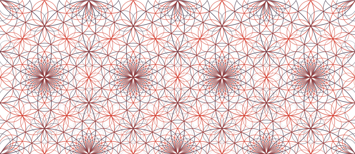
![ResourceFunction["SchmidtArrangements"][-15, "MinCurvature" -> 0, "MaxCurvature" -> 20, "Color" -> {"ColorSaul", {1, 0}},
"XMax" -> 10.0, "YMax" -> 2.0,
"Filter" -> Rectangle[{-0.1, -0.1}, {5.1, Sqrt[15.0] + 0.1}],
"Circle" -> False, PlotRange -> {{0, 5}, {0, Sqrt[15.0]/2.0}}, ImageSize -> Large]](https://www.wolframcloud.com/obj/resourcesystem/images/330/33072f77-33e8-4cd6-9838-8fe0b21d493e/3b86314ae344a78d.png)
![precomputed = ResourceFunction["SchmidtArrangements"][-1, "MaxCurvature" -> 100, "Precompute" -> True]; // ResourceFunction[
ResourceObject[<|"Name" -> "EchoTiming", "ShortName" -> "EchoTiming", "UUID" -> "b6064c2f-0a91-4537-8ac3-ef527c794326", "ResourceType" -> "Function", "Version" -> "1.0.0", "Description" -> "Print the timing for an evaluation and return the result", "RepositoryLocation" -> URL[
"https://www.wolframcloud.com/obj/resourcesystem/api/1.0"], "SymbolName" -> "GeneralUtilities`EchoTiming", "FunctionLocation" -> CloudObject[
"https://www.wolframcloud.com/objects/579490e1-7faa-43b0-a99d-0f4188efc7c8"]|>, ResourceSystemBase -> Automatic]]](https://www.wolframcloud.com/obj/resourcesystem/images/330/33072f77-33e8-4cd6-9838-8fe0b21d493e/5daa50440d7c506d.png)
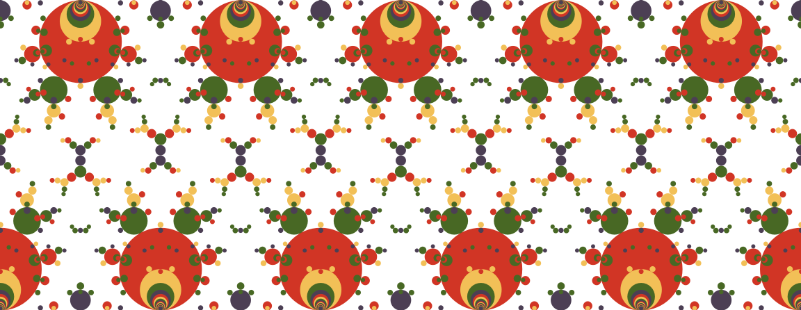
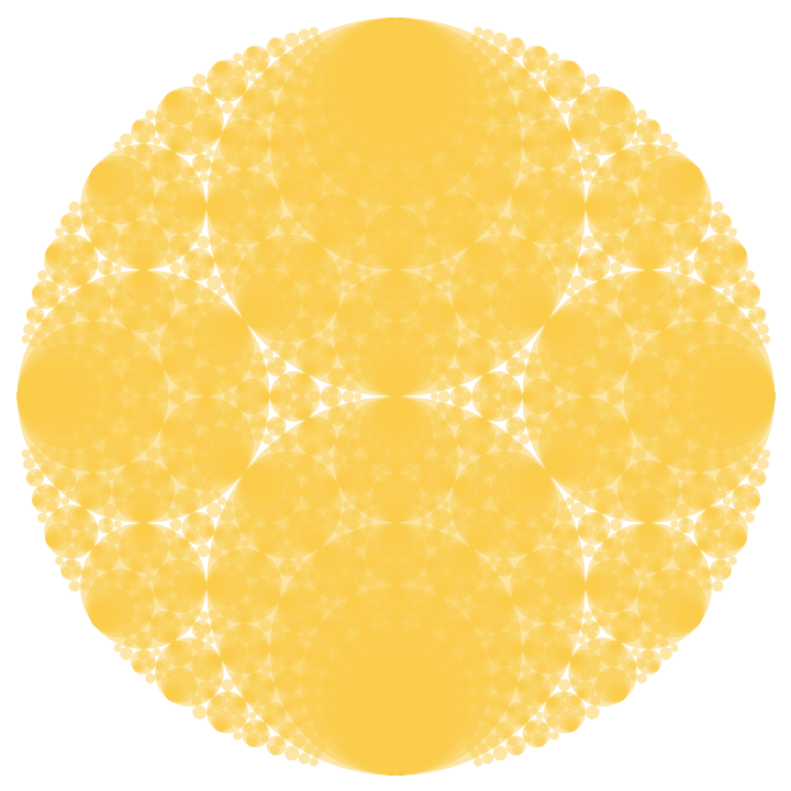
![ResourceFunction["SchmidtArrangements"][precomputed, "Circle" -> False, "Containment" -> False, "MinCurvature" -> 2, "MaxCurvature" -> 100, "Color" -> {"Color24", {1, 4}}] // ResourceFunction[
ResourceObject[<|"Name" -> "EchoTiming", "ShortName" -> "EchoTiming", "UUID" -> "b6064c2f-0a91-4537-8ac3-ef527c794326", "ResourceType" -> "Function", "Version" -> "1.0.0", "Description" -> "Print the timing for an evaluation and return the result", "RepositoryLocation" -> URL[
"https://www.wolframcloud.com/obj/resourcesystem/api/1.0"], "SymbolName" -> "GeneralUtilities`EchoTiming", "FunctionLocation" -> CloudObject[
"https://www.wolframcloud.com/objects/579490e1-7faa-43b0-a99d-0f4188efc7c8"]|>, ResourceSystemBase -> Automatic]]](https://www.wolframcloud.com/obj/resourcesystem/images/330/33072f77-33e8-4cd6-9838-8fe0b21d493e/30fa637cf4bc1c7e.png)
![precomputed2 = ResourceFunction["SchmidtArrangements"][-1, "MaxCurvature" -> 100, "Precompute" -> True]; // ResourceFunction[
ResourceObject[<|"Name" -> "EchoTiming", "ShortName" -> "EchoTiming", "UUID" -> "b6064c2f-0a91-4537-8ac3-ef527c794326", "ResourceType" -> "Function", "Version" -> "1.0.0", "Description" -> "Print the timing for an evaluation and return the result", "RepositoryLocation" -> URL[
"https://www.wolframcloud.com/obj/resourcesystem/api/1.0"], "SymbolName" -> "GeneralUtilities`EchoTiming", "FunctionLocation" -> CloudObject[
"https://www.wolframcloud.com/objects/579490e1-7faa-43b0-a99d-0f4188efc7c8"]|>, ResourceSystemBase -> Automatic]]](https://www.wolframcloud.com/obj/resourcesystem/images/330/33072f77-33e8-4cd6-9838-8fe0b21d493e/12bc3dbefc581c83.png)
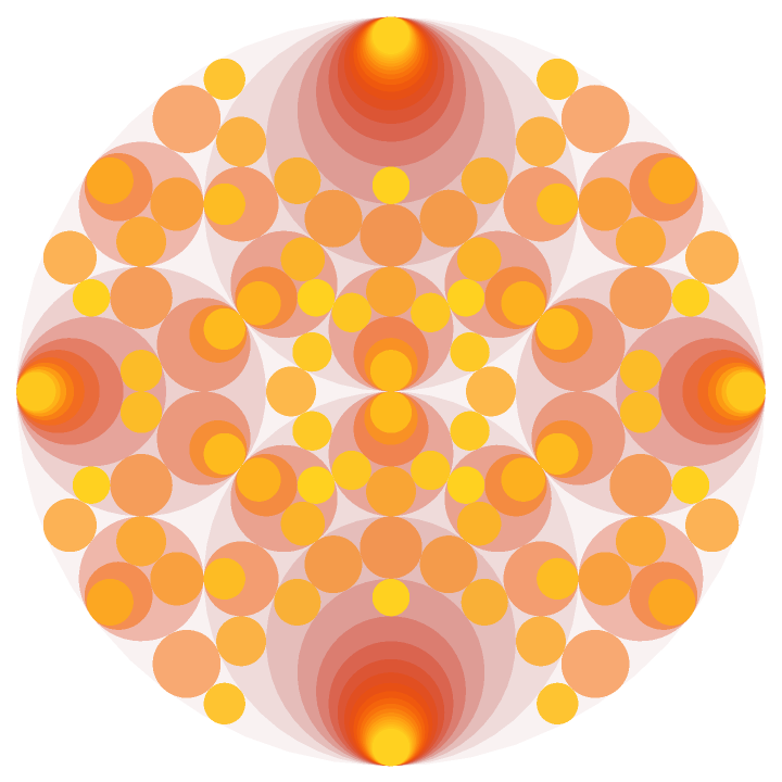
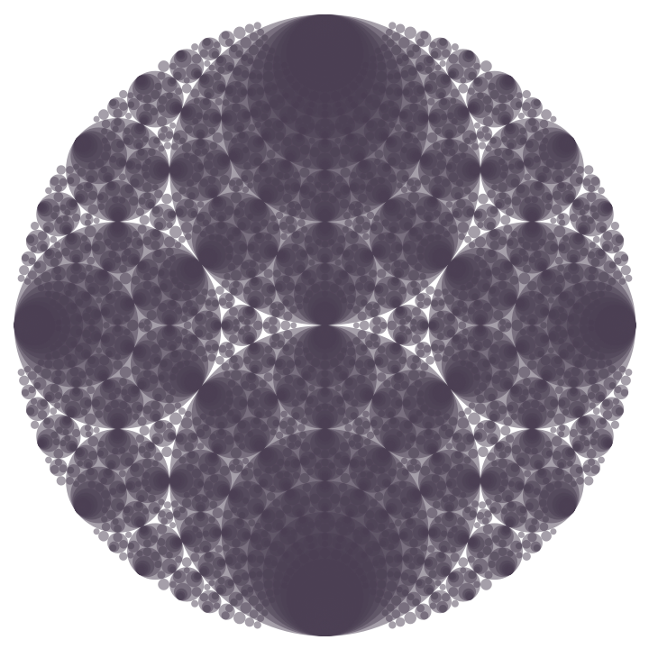
![ResourceFunction["SchmidtArrangements"][precomputed2, "Circle" -> False, "Color" -> {"Color92", {0, 0}},
"Transparency" -> 0.5, "MinCurvature" -> 2, "MaxCurvature" -> 100] // ResourceFunction[
ResourceObject[<|"Name" -> "EchoTiming", "ShortName" -> "EchoTiming", "UUID" -> "b6064c2f-0a91-4537-8ac3-ef527c794326", "ResourceType" -> "Function", "Version" -> "1.0.0", "Description" -> "Print the timing for an evaluation and return the result", "RepositoryLocation" -> URL[
"https://www.wolframcloud.com/obj/resourcesystem/api/1.0"], "SymbolName" -> "GeneralUtilities`EchoTiming", "FunctionLocation" -> CloudObject[
"https://www.wolframcloud.com/objects/579490e1-7faa-43b0-a99d-0f4188efc7c8"]|>, ResourceSystemBase -> Automatic]]](https://www.wolframcloud.com/obj/resourcesystem/images/330/33072f77-33e8-4cd6-9838-8fe0b21d493e/09f952d7e1b13e1e.png)
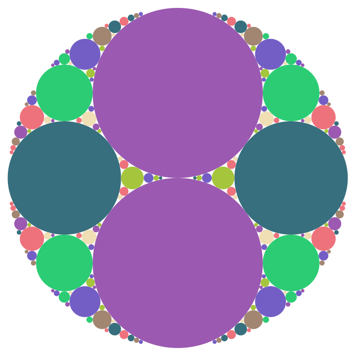
![ResourceFunction["SchmidtArrangements"][precomputed2, "Circle" -> False, "Color" -> {"ColorA", {0, 0}},
"Transparency" -> 0.5, "MinCurvature" -> 2, "MaxCurvature" -> 100] // ResourceFunction[
ResourceObject[<|"Name" -> "EchoTiming", "ShortName" -> "EchoTiming", "UUID" -> "b6064c2f-0a91-4537-8ac3-ef527c794326", "ResourceType" -> "Function", "Version" -> "1.0.0", "Description" -> "Print the timing for an evaluation and return the result", "RepositoryLocation" -> URL[
"https://www.wolframcloud.com/obj/resourcesystem/api/1.0"], "SymbolName" -> "GeneralUtilities`EchoTiming", "FunctionLocation" -> CloudObject[
"https://www.wolframcloud.com/objects/579490e1-7faa-43b0-a99d-0f4188efc7c8"]|>, ResourceSystemBase -> Automatic]]](https://www.wolframcloud.com/obj/resourcesystem/images/330/33072f77-33e8-4cd6-9838-8fe0b21d493e/23c53d02010a6c2e.png)
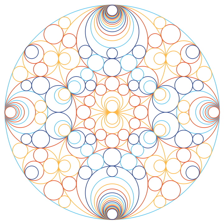
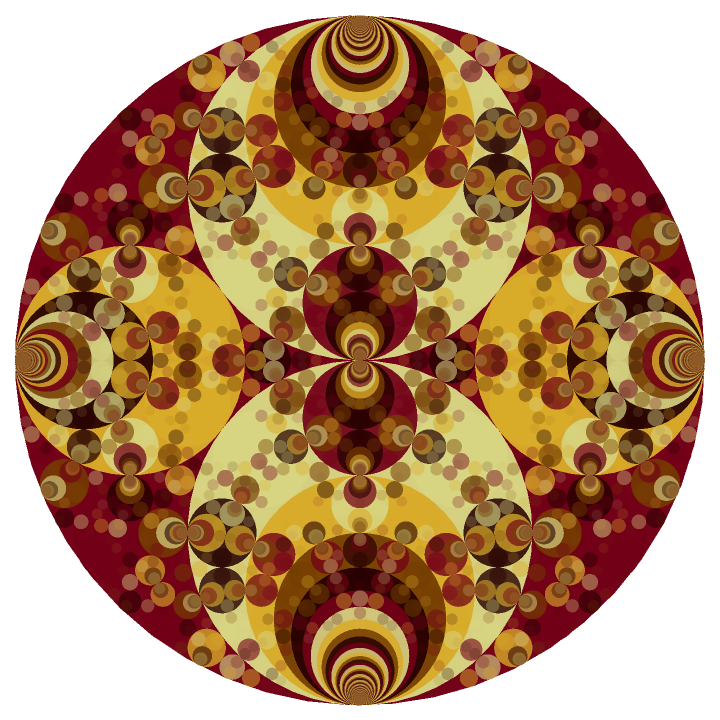
![ResourceFunction["SchmidtArrangements"][precomputed2, "Circle" -> False, "Color" -> {"Color5", {1, 0}},
"Transparency" -> "Increasing", "MinCurvature" -> 0, "MaxCurvature" -> 75,
"Filter" -> Circle[{0., 0.5}, Sqrt[0.25]]] // ResourceFunction[
ResourceObject[<|"Name" -> "EchoTiming", "ShortName" -> "EchoTiming", "UUID" -> "b6064c2f-0a91-4537-8ac3-ef527c794326", "ResourceType" -> "Function", "Version" -> "1.0.0", "Description" -> "Print the timing for an evaluation and return the result", "RepositoryLocation" -> URL[
"https://www.wolframcloud.com/obj/resourcesystem/api/1.0"], "SymbolName" -> "GeneralUtilities`EchoTiming", "FunctionLocation" -> CloudObject[
"https://www.wolframcloud.com/objects/579490e1-7faa-43b0-a99d-0f4188efc7c8"]|>, ResourceSystemBase -> Automatic]]](https://www.wolframcloud.com/obj/resourcesystem/images/330/33072f77-33e8-4cd6-9838-8fe0b21d493e/7f7807035c9df594.png)
![(* Evaluate this cell to get the example input *) CloudGet["https://www.wolframcloud.com/obj/578b0790-dcc6-4c11-a459-6c075c13233d"]](https://www.wolframcloud.com/obj/resourcesystem/images/330/33072f77-33e8-4cd6-9838-8fe0b21d493e/107c954cfa9fbe77.png)
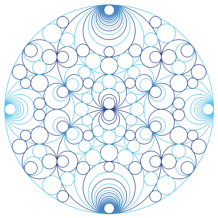
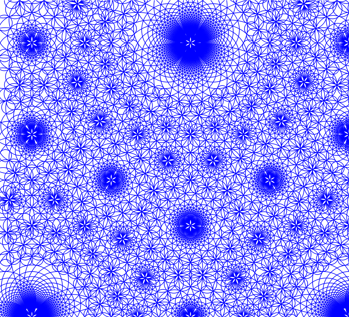
![ResourceFunction["SchmidtArrangements"][-3, "MinCurvature" -> 0, "MaxCurvature" -> 30, "Color" -> Blue,
"Filter" -> Rectangle[{-0.1, -0.1}, {1.1, 1.1}], PlotRange -> {{-0.1, 1}, {0, 1.0}}, ImageSize -> Large]](https://www.wolframcloud.com/obj/resourcesystem/images/330/33072f77-33e8-4cd6-9838-8fe0b21d493e/456d6094c34dcc4a.png)
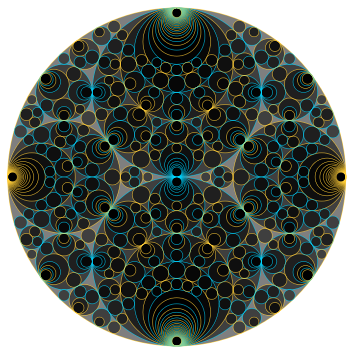
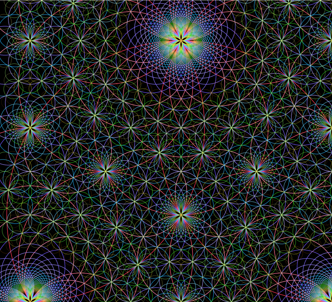
![ResourceFunction["SchmidtArrangements"][pre, "MinCurvature" -> 0, "MaxCurvature" -> 30, "Color" -> ColorData["BrightBands"], "Transparency" -> "Increasing",
"Filter" -> Rectangle[{-0.1, -0.1}, {1.1, 1.1}], PlotRange -> {{-0.1, 1}, {0, 1.0}}, ImageSize -> Large, Background -> Black]](https://www.wolframcloud.com/obj/resourcesystem/images/330/33072f77-33e8-4cd6-9838-8fe0b21d493e/60abcb00620f5b7c.png)
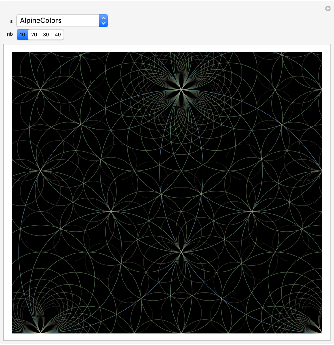
![Manipulate[
ResourceFunction["SchmidtArrangements"][pre, "MinCurvature" -> 0, "MaxCurvature" -> nb, "Color" -> ColorData[s], "Transparency" -> "Increasing",
"Filter" -> Rectangle[{-0.1, -0.1}, {1.1, 1.1}], PlotRange -> {{-0.1, 1}, {0, 1.0}}, ImageSize -> Large, Background -> Black],
{s, ColorData["Gradients"]}, {{nb, 10}, {10, 20, 30, 40}}
]](https://www.wolframcloud.com/obj/resourcesystem/images/330/33072f77-33e8-4cd6-9838-8fe0b21d493e/54f71d756ed4f10c.png)