Wolfram Function Repository
Instant-use add-on functions for the Wolfram Language
Function Repository Resource:
Make a Saunders plot of a function
ResourceFunction["SaundersDigitPlot"][f,b,k,{x,xmin,xmax},{y,ymin,ymax}] makes a Saunders plot of the kth base‐b digit of f as a function of x and y. | |
ResourceFunction["SaundersDigitPlot"][f,b,k,{x,y}∈reg] takes the variables {x,y} to be in the geometric region reg. |
A Saunders plot of a function's first base-10 digit to the right of the decimal point:
| In[1]:= |
| Out[1]= | 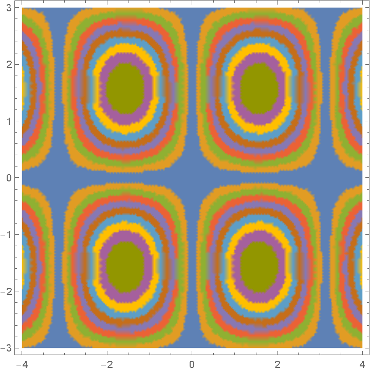 |
Visualize the third binary digit:
| In[2]:= |
| Out[2]= | 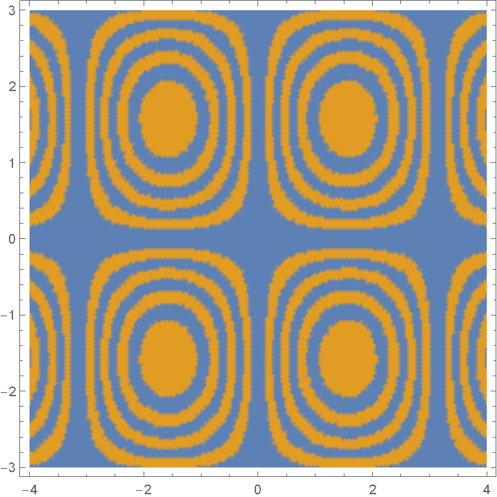 |
Use a different color scheme and legend:
| In[3]:= |
| Out[3]= | 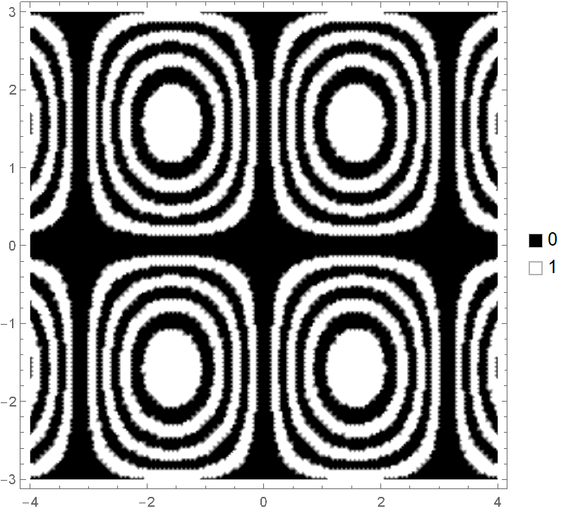 |
Use a non-integer base:
| In[4]:= |
| Out[4]= | 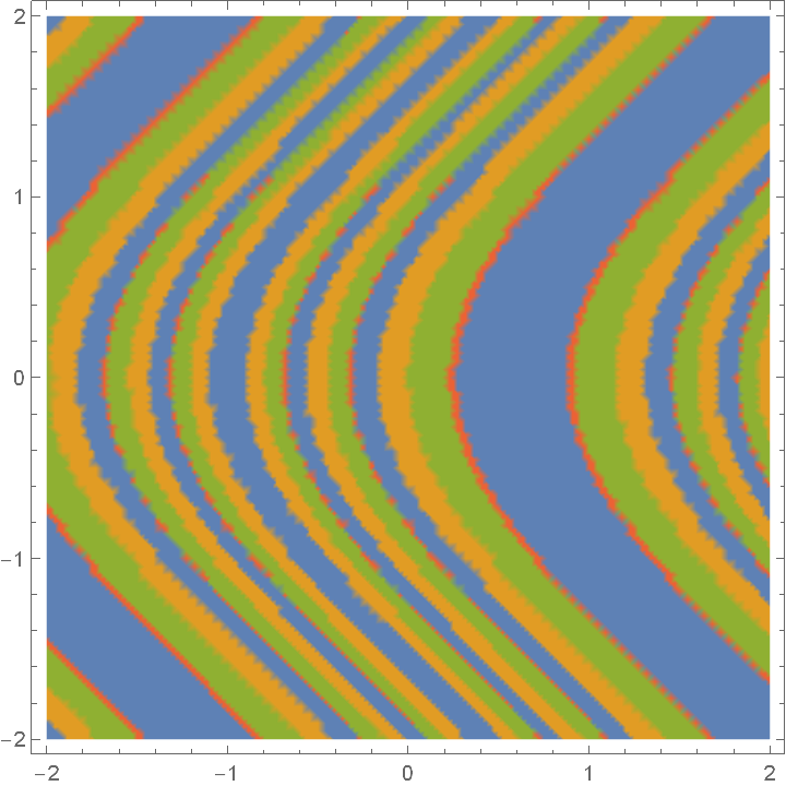 |
Use PlotPoints and MaxRecursion to control adaptive sampling:
| In[5]:= |
| Out[5]= | 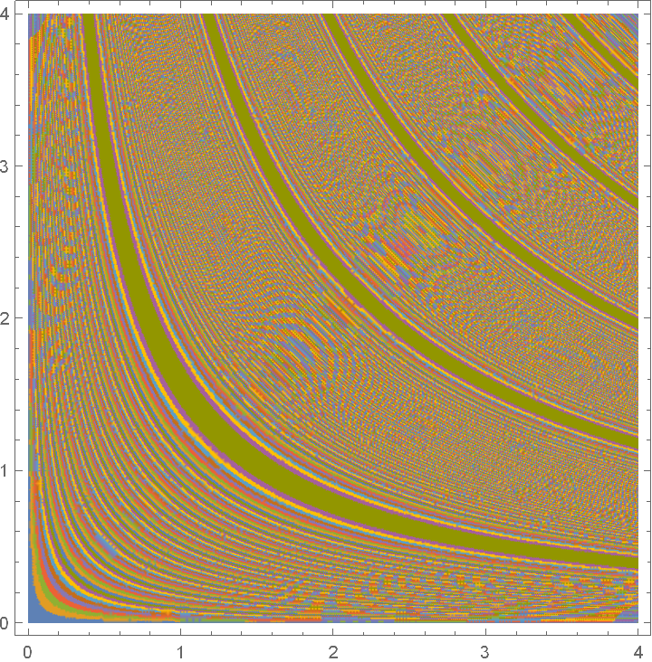 |
The domain may be specified by a region:
| In[6]:= |
| Out[6]= | 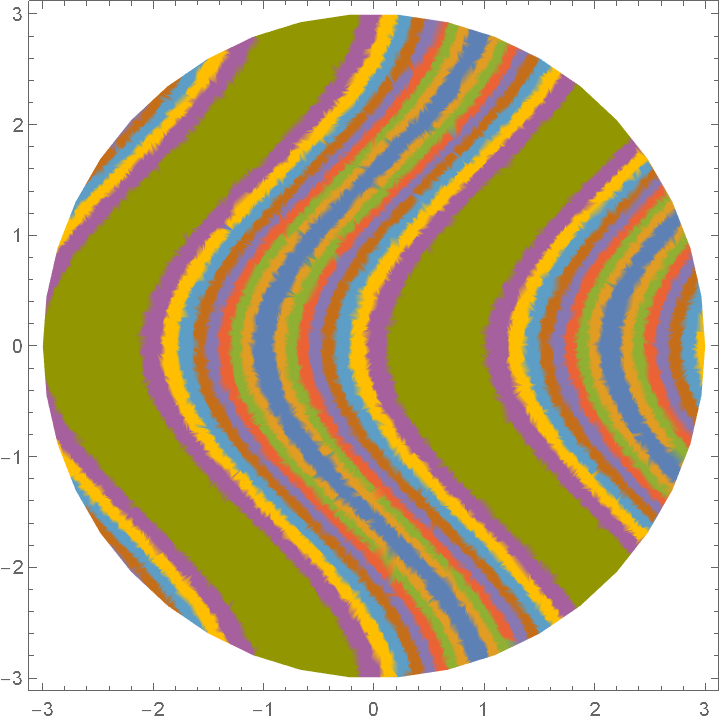 |
Explicitly specify a color function:
| In[7]:= |
| Out[7]= | 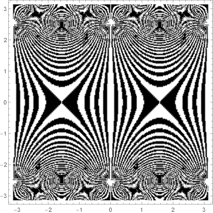 |
Use an indexed color:
| In[8]:= |
| Out[8]= | 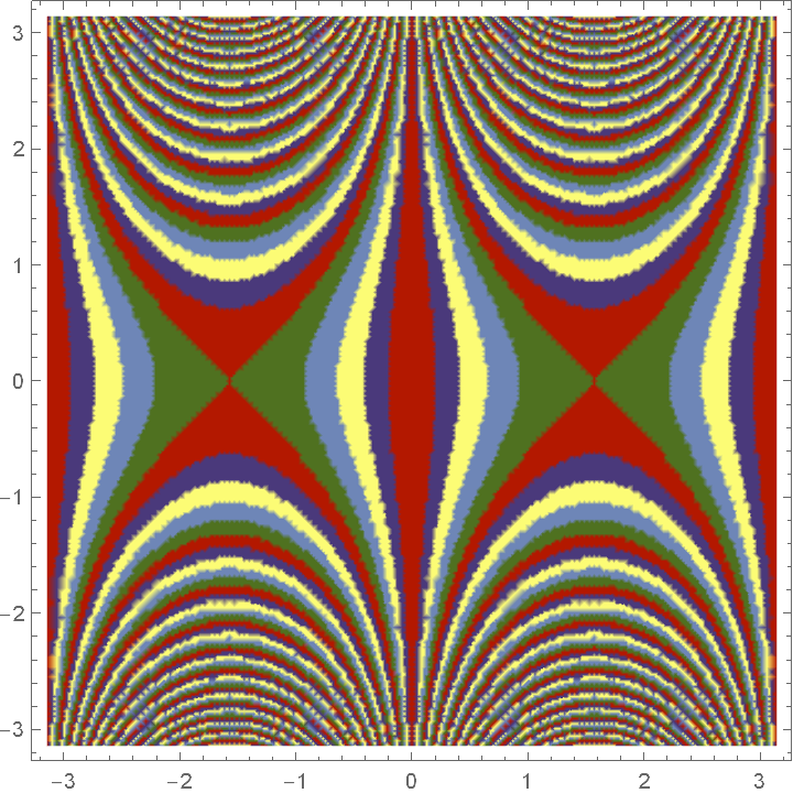 |
Use a named color gradient:
| In[9]:= |
| Out[9]= | 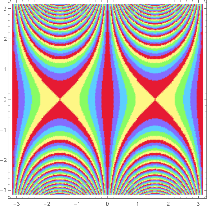 |
Show a legend for the digits:
| In[10]:= |
| Out[10]= | 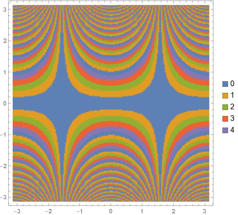 |
Use Placed to change legend position:
| In[11]:= |
| Out[11]= | 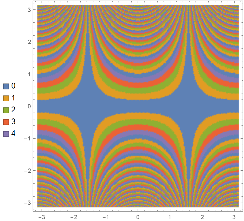 |
Visualize the base-5 digits of a doubly periodic function:
| In[12]:= |
| Out[12]= | 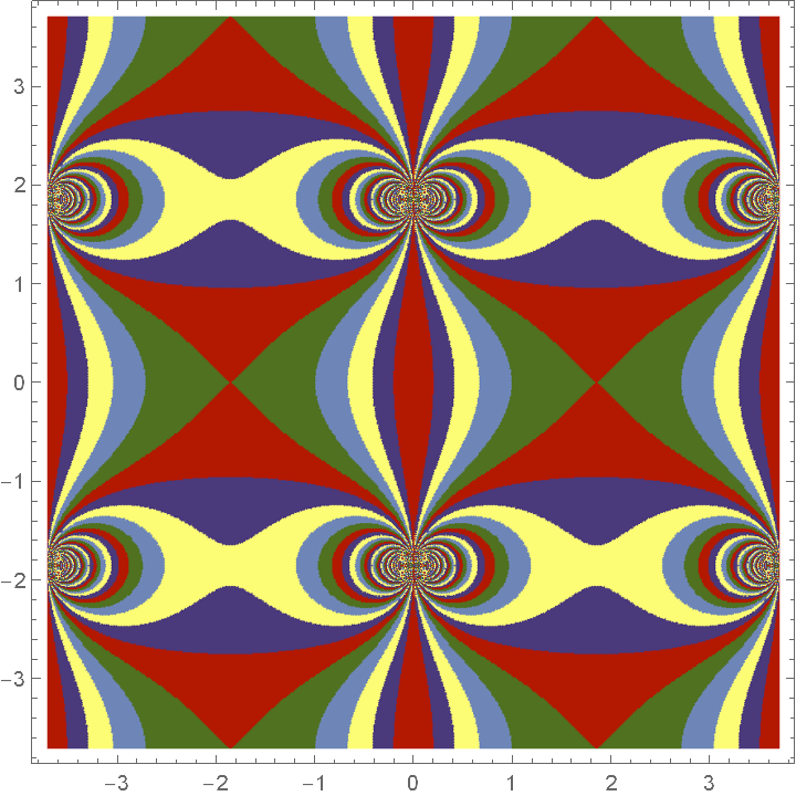 |
This work is licensed under a Creative Commons Attribution 4.0 International License