Wolfram Function Repository
Instant-use add-on functions for the Wolfram Language
Function Repository Resource:
Plot a ruled surface
ResourceFunction["RuledSurfacePlot"][c1,c2,u] plots a ruled surface from the curves c1 and c2 that are parameterized by the variable u. | |
ResourceFunction["RuledSurfacePlot"][c1,c2,{u,umin,umax},{v,vmin,vmax}] plots a ruled surface with u varying from umin to umax and v varying from vmin to vmax. |
A simple ruled surface:
| In[1]:= | ![Show[ResourceFunction[
"RuledSurfacePlot"][{Cos[u], Sin[u], 0}, {Sin[u], Cos[u], 1}, u], ParametricPlot3D[{{Cos[u], Sin[u], 0}, {Cos[u], Sin[u], g}}, {u, 0, 2 \[Pi]}]]](https://www.wolframcloud.com/obj/resourcesystem/images/700/700fa273-0c8f-4323-93bd-309c7809c1e7/496741e0e8994d79.png) |
| Out[1]= | 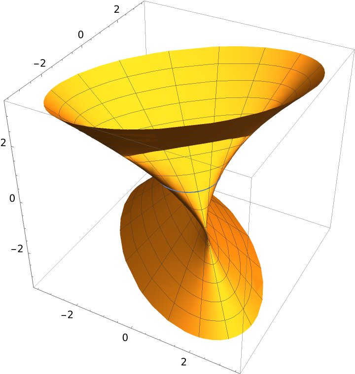 |
This Manipulate shows how the surface is generated, the right line moves around intersecting the two curves, for definite values of u and v:
| In[2]:= | ![Manipulate[
Show[ResourceFunction[
"RuledSurfacePlot"][{Cos[u], Sin[u], 0}, {Sin[u], Cos[u], 1}, {u, -$MachineEpsilon, uf}, {v, -3, 2}, MeshStyle -> Directive[AbsoluteThickness[0.5], Opacity[0.2]], PlotStyle -> Opacity[0.1], PlotRange -> 4],
ParametricPlot3D[{{Cos[u], Sin[u], 0}, {Cos[u], Sin[u], 0} + vf {Sin[u], Cos[u], 1}}, {u, 0, 2 \[Pi]}, PlotStyle -> AbsoluteThickness[4]],
Graphics3D[{Directive[AbsoluteThickness[3], ColorData[97, 3]], Line[{{Cos[uf], Sin[uf], 0}, {Cos[uf], Sin[uf], 0} + vf {Sin[uf], Cos[uf], 1}}]}]],
{{uf, 2 \[Pi]}, 0, 2 \[Pi]}, {vf, -3, 2}, SaveDefinitions -> True, ControlPlacement -> Top]](https://www.wolframcloud.com/obj/resourcesystem/images/700/700fa273-0c8f-4323-93bd-309c7809c1e7/15bb69824076d51f.png) |
| Out[2]= | 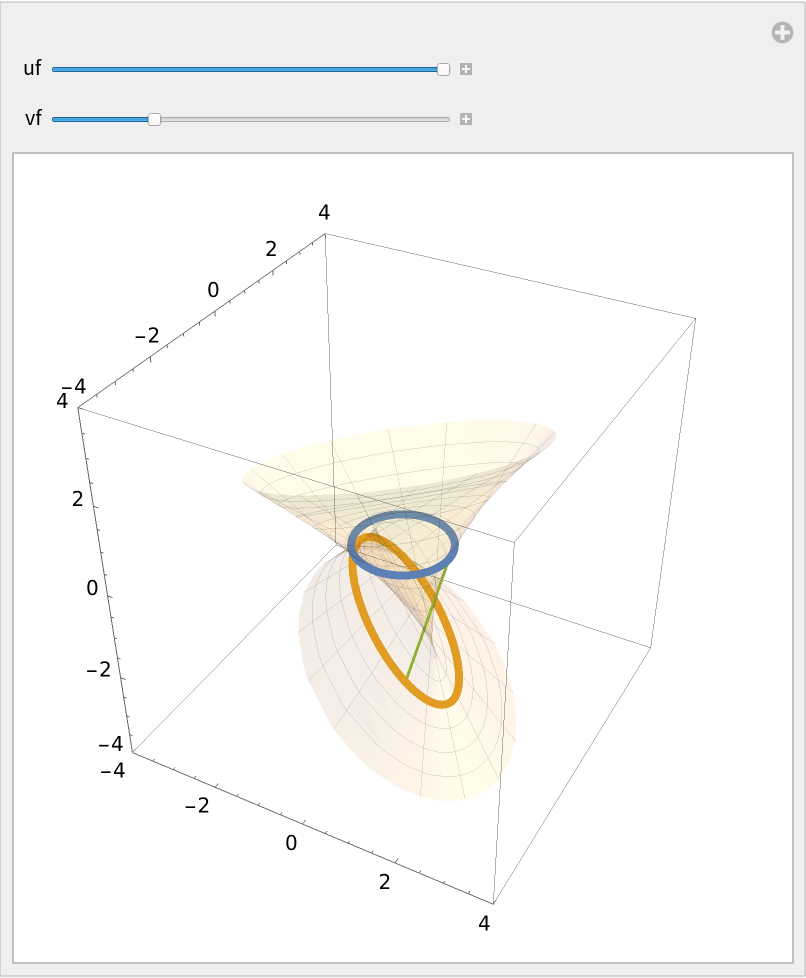 |
Modify the default ranges:
| In[3]:= |
| Out[3]= | 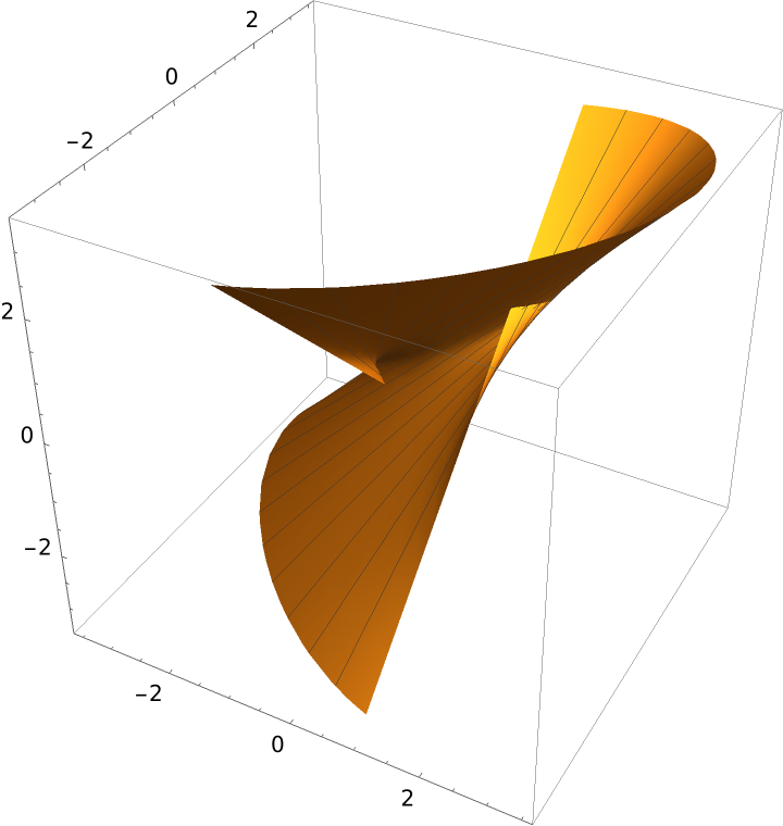 |
Modify the options for enhanced viewing:
| In[4]:= | ![ResourceFunction[
"RuledSurfacePlot"][{Cos[u], Sin[u], 0}, {Sin[u], Cos[u], 1}, u, PlotStyle -> Directive[Opacity[0.5], Yellow], MeshFunctions -> {#4 &}, MeshShading -> {Red, Automatic}]](https://www.wolframcloud.com/obj/resourcesystem/images/700/700fa273-0c8f-4323-93bd-309c7809c1e7/169531072dcfe76a.png) |
| Out[4]= |  |
Plot the generalized hyperbolic paraboloid:
| In[5]:= | ![With[{a = 1, b = -1}, ResourceFunction[
"RuledSurfacePlot"][{a u, 0, u^2}, {0, #, 2 u}, {u, -1, 1}, {v, -1, 1}, Mesh -> {30, 0}, BoxRatios -> {1, 1, 1}, PlotRange -> All]] & /@ {-1, 1}](https://www.wolframcloud.com/obj/resourcesystem/images/700/700fa273-0c8f-4323-93bd-309c7809c1e7/77cc449cd5375eb8.png) |
| Out[5]= | 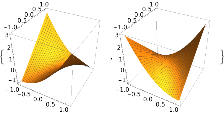 |
Define the Plücker conoid:
| In[6]:= |
| Out[6]= |
Plot the conoid:
| In[7]:= |
| Out[7]= | 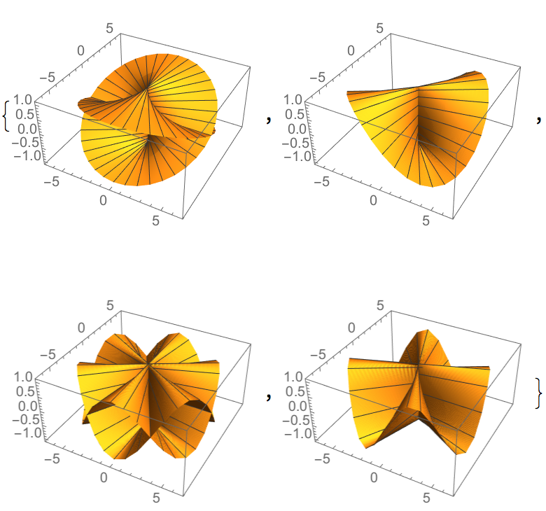 |
The Möbius strip as a ruled surface:
| In[8]:= |
| Out[8]= |  |
A representation of the director curve c2(u):
| In[9]:= | ![Show[ParametricPlot3D[{Cos[u/2] Cos[u], Cos[u/2] Sin[u], Sin[u/2]}, {u, 0, 4 \[Pi]}, ViewPoint -> {2, 2, 2}, PlotRange -> All], ParametricPlot3D[ {Cos[v] Cos[u], Cos[v] Sin[u], Sin[v]}, {u, 3 \[Pi]/8, 13 \[Pi]/8}, {v, -\[Pi]/2, \[Pi]/2}, PlotStyle -> Opacity[.5]]]](https://www.wolframcloud.com/obj/resourcesystem/images/700/700fa273-0c8f-4323-93bd-309c7809c1e7/5c8a9934dbee1129.png) |
| Out[9]= | 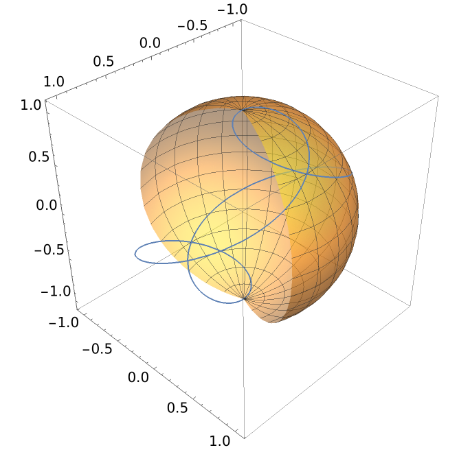 |
An elliptical hyperboloid is doubly ruled because it can be parametrized in two ways:
| In[10]:= |
The "minus" chart could easily have been defined in terms of the "plus" one:
| In[11]:= |
| Out[11]= |
Plot both cases:
| In[12]:= | ![With[{a = 1, b = 2, c = 3},
GraphicsRow[{ResourceFunction[
"RuledSurfacePlot"][{a Cos[u], b Sin[u], 0}, {-a Sin[u], b Cos[u], c}, {u, 0, 3 \[Pi]/2}, {v, -1.5, 1.5}, PlotStyle -> Opacity[.5], Mesh -> {30, 0}],
ResourceFunction[
"RuledSurfacePlot"][{a Cos[u], b Sin[u], 0}, {a Sin[u], -b Cos[u],
c}, {u, 0, 3 \[Pi]/2}, {v, -1.5, 1.5}, PlotStyle -> Opacity[.5],
Mesh -> {20, 0}]}]]](https://www.wolframcloud.com/obj/resourcesystem/images/700/700fa273-0c8f-4323-93bd-309c7809c1e7/3a9da840ab39acfe.png) |
| Out[12]= | 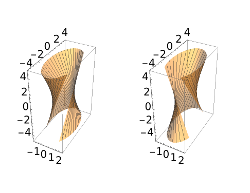 |
The Gaussian curvature of a ruled surface is everywhere nonpositive:
| In[13]:= |
| Out[13]= |
| In[14]:= |
| Out[14]= |
This plot exhibits its minima, corresponding to regions which are especially distorted:
| In[15]:= |
| Out[15]= | 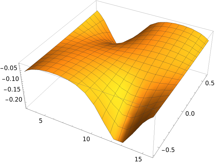 |
Generalized cylinders and cones have the form of a ruled surface:
| In[16]:= |
A figure-eight curve:
| In[17]:= |
Parametrizations of a generalized cylinder and cone using a figure-eight curve:
| In[18]:= |
| Out[18]= |
| In[19]:= |
| Out[19]= |
Plot the surfaces:
| In[20]:= | ![GraphicsRow[{ResourceFunction[
"RuledSurfacePlot"][{Sin[u], Cos[u] Sin[u], 0}, {0, 1, 1},
{u, 0, 2 \[Pi]}, {v, 0, 2}, PlotPoints -> {40, 15}, Mesh -> {30, {0}}],
ResourceFunction[
"RuledSurfacePlot"][{0, 0, 0}, {1/2 + 2 Sin[u], 1/2 + 2 Cos[u] Sin[u], 2 }, {u, 0, 2 \[Pi]}, {v, -3, 3},
PlotPoints -> {40, 15}, Mesh -> {30, 0}]}]](https://www.wolframcloud.com/obj/resourcesystem/images/700/700fa273-0c8f-4323-93bd-309c7809c1e7/2c4344342ceb110f.png) |
| Out[20]= | 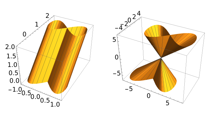 |
If the Gaussian curvature of a ruled surface is everywhere zero, then it is said to be a flat surface:
| In[21]:= |
| Out[21]= |
| In[22]:= |
| Out[22]= |
The tangent developable of a space curve α is a ruled surface, whose director curve is the unit tangent vector field to α:
| In[23]:= |
| Out[23]= |
| In[24]:= |
| Out[24]= |
| In[25]:= |
| Out[25]= |  |
| In[26]:= |
| Out[26]= | 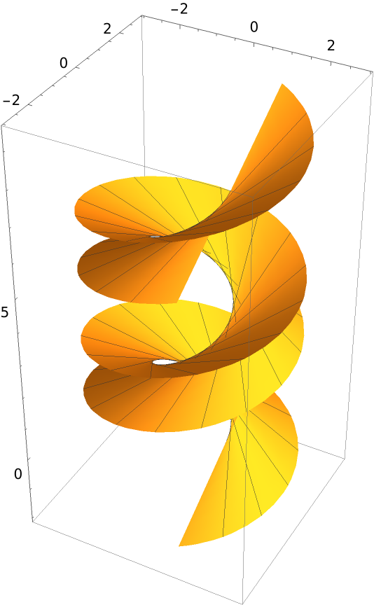 |
This work is licensed under a Creative Commons Attribution 4.0 International License