Function Repository Resource:

RiemannSum

Compute information related to a Riemann sum

Contributed by: Wolfram|Alpha Math Team, Jeremy Stratton-Smith

ResourceFunction["RiemannSum"][expr,{x,x_min,x_max,n},m,method]

computes an association of data related to the Riemann sum of expr specified by method on the domain x_min<=x<=x_max partitioned into n intervals of equal length.

ResourceFunction["RiemannSum"][expr,{x,x_min,x_max,n},m,method,property]

computes the information specified by property related to the Riemann sum of expr on the given domain.

ResourceFunction["RiemannSum"][expr,{x,x_min,x_max,n},m,All,property]

computes the information specified by property for all Riemann sum methods.

ResourceFunction["RiemannSum"][expr,{x,x_min,x_max,n},m]

computes all properties of the Riemann sum for all methods.

Details

The input expr is expected to be the kind of input that Plot accepts (e.g. Sin[x], x², etc.).

The input method can be any of All, "Left", "Right", "Midpoint" or "Trapezoidal" and defaults to All. This input determines the value to be taken in each of the intervals of the Riemann sum that is used for computing the sum.

The input property can be any of the following:

"InactiveSum"

inactivated Sum over the input variable m, where the summand is determined by the method and n.

"Sum"

activated sum

"InactiveIntegral"

inactivated integral that the given Riemann sum approximates

"Integral"

actual value of the integral

"AbsoluteError"

absolute error between the integral value and the sum value

"RelativeError"

relative error between the integral value and the sum value

"Plot"

plot showing the curve and the areas that are computed as the terms of the Riemann sum

Dataset

formatted output of all properties as a Dataset

A Riemann sum is an approximation of an integral and one of the first ways that a definite integral is introduced and defined.

Examples

Basic Examples (2)

Compute information related to a left Riemann sum:

In[1]:=

$ResourceFunction[ "RiemannSum", ResourceSystemBase -> "https://www.wolframcloud.com/obj/resourcesystem/api/1.0"][E^x, {x, 0, 2, 10}, n, "Left"]$

Out[1]=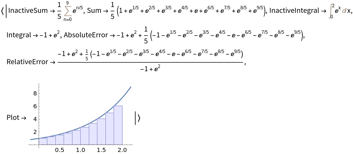

Alternatively, compute just a particular property:

In[2]:=

$ResourceFunction[ "RiemannSum", ResourceSystemBase -> "https://www.wolframcloud.com/obj/resourcesystem/api/1.0"][E^x, {x, 0, 2, 10}, n, "Left", "Plot"]$

Out[2]=

Scope (2)

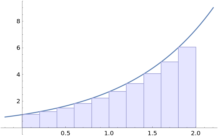For easy comparison, return only a particular property for all four methods:

In[3]:=

$expr = -x + x^3; ResourceFunction[ "RiemannSum", ResourceSystemBase -> "https://www.wolframcloud.com/obj/resourcesystem/api/1.0"][expr, {x, -1, 1, 10}, n, All, "Plot"]$

Out[3]=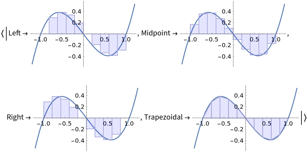

Check that in this special case, all four methods return the same result:

In[4]:=

Out[4]=

RiemannSum can also compute with a symbolic number of intervals:

In[5]:=

$data = ResourceFunction[ "RiemannSum", ResourceSystemBase -> "https://www.wolframcloud.com/obj/resourcesystem/api/1.0"][x^2, {x, 0, 1, m}, n, "Left"]$

Out[5]=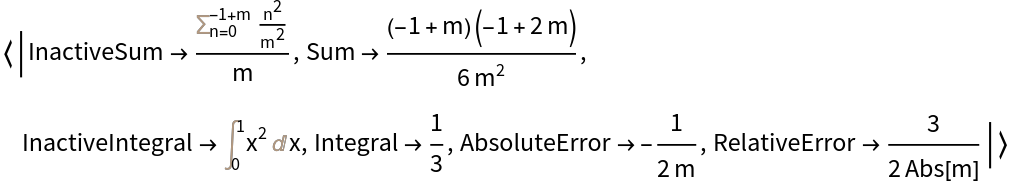

Compute the limiting behavior of the sum as the number of intervals goes to infinity:

In[6]:=

Out[6]=

Show that this matches the actual value of the definite integral:

In[7]:=

Out[7]=

Applications (3)

Show that in the finite case, the four methods may return differently:

In[8]:=

$ResourceFunction[ "RiemannSum", ResourceSystemBase -> "https://www.wolframcloud.com/obj/resourcesystem/api/1.0"][x^3, {x, 0, 1, 20}, n, All, "Sum"]$

Out[8]=

This can be seen symbolically as well:

In[9]:=

$data = ResourceFunction[ "RiemannSum", ResourceSystemBase -> "https://www.wolframcloud.com/obj/resourcesystem/api/1.0"][x^3, {x, 0, 1, m}, n, All, "Sum"]$

Out[9]=

But in the limit, they are equivalent, and are equivalent to computing the definite integral:

In[10]:=

Out[10]=

In[11]:=

$integral = ResourceFunction[ "RiemannSum", ResourceSystemBase -> "https://www.wolframcloud.com/obj/resourcesystem/api/1.0"][x^3, {x, 0, 1, m}, n, "Left", "Integral"]; AllTrue[Values[limits], # == integral &]$

Out[11]=

Properties and Relations (2)

For a given curve, one of the "Left", "Right", "Midpoint" or "Trapezoidal" Riemann sums will be the best approximation for the definite integral:

In[12]:=

$ResourceFunction[ "RiemannSum", ResourceSystemBase -> "https://www.wolframcloud.com/obj/resourcesystem/api/1.0"][ 2 + 10 x - 15 x^2 + 5 x^3, {x, 0, 3/2, 3}, n, All, "AbsoluteError"]$

Out[12]=

In[13]:=

Out[13]=

For curves that are concave up, the "Left" method will under-approximate the definite integral, while the "Right" and "Trapezoidal" methods will over-approximate:

In[14]:=

$data = ResourceFunction[ "RiemannSum", ResourceSystemBase -> "https://www.wolframcloud.com/obj/resourcesystem/api/1.0"][x^2, {x, 0, 3, 10}, n, "Left"]; data["Integral"] - data["Sum"]$

Out[14]=

In[15]:=

$data = ResourceFunction[ "RiemannSum", ResourceSystemBase -> "https://www.wolframcloud.com/obj/resourcesystem/api/1.0"][x^2, {x, 0, 3, 10}, n, "Right"]; data["Integral"] - data["Sum"]$

Out[15]=

Publisher

Wolfram|Alpha Math Team

Version History

2.0.0 – 23 March 2023
1.0.0 – 02 June 2021

Related Resources

License Information

This work is licensed under a Creative Commons Attribution 4.0 International License

Wolfram Function Repository

RiemannSum

Details