Function Repository Resource:

RichardsonExtrapolate

Calculate an accelerated version of a symbolic sequence

Contributed by: József Konczer

ResourceFunction["RichardsonExtrapolate"][expr,m,k,n]

gives the m^th order Richardson extrapolation of expr with respect to k using n as the independent variable of the transformed sequence.

ResourceFunction["RichardsonExtrapolate"][expr,{g₁,…,g_m},k,n]

uses auxiliary sequences g₁,…,g_m.

ResourceFunction["RichardsonExtrapolate"][list, m]

gives the m^th order Richardson extrapolation of list.

ResourceFunction["RichardsonExtrapolate"][list,{g₁,…,g_m}]

uses auxiliary lists g₁,…,g_m.

Details and Options

Richardson extrapolation is a linear sequence transfomation. In the simplest case, it projects out

constituents from the sequence A[n], which can expressed by Cramer’s rule, or by the explicit formula below:

The method can be generalized by introducing auxiliary sequences g₁[n],g₂[n],…,g_M[n], which can be projected out by using Cramer's rule (or using the so-called BrezinskiE) shown below:

For more info about BrezinskiE (i.e. the E-Algorithm), see references [3] and [2].

ResourceFunction["RichardsonExtrapolate"] can take following options:

Method

"BrezinskiE"

method to use

"MinWorkingPrecision"

minimum precision to use

Supported options for Method are "BrezinskiE", "LinearSolve" and "Cramer".

If an entry has less precision than the value of "MinWorkingPrecision", then its precision is set to "MinWorkingPrecision" by SetPrecision.

ResourceFunction["RichardsonExtrapolate"] uses Block to localize values or variables.

Examples

Basic Examples (4)

Find a sequence which converges to the same limit faster than the input sequence:

In[1]:=

Out[1]=

Given the first few terms of a sequence, find terms of another sequence with accelerated convergence:

In[2]:=

Out[2]=

Accelerate the convergence of the sequence 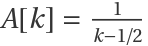by specifying the auxiliary sequences:

In[3]:=

$ResourceFunction["RichardsonExtrapolate"][1/( k - 1/2), {1/k, 1/k^2}, k, n]$

Out[3]=

Give a finite list and specify auxiliary lists:

In[4]:=

Out[4]=

Options (5)

Method (3)

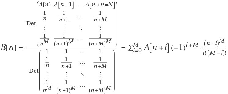
The default Method is "BrezinskiE", which uses a recursive definition:

In[5]:=

$be = ResourceFunction["RichardsonExtrapolate"][1/( k - 1/2), {1/k, 1/k^2}, k, n, Method -> "BrezinskiE"]$

Out[5]=

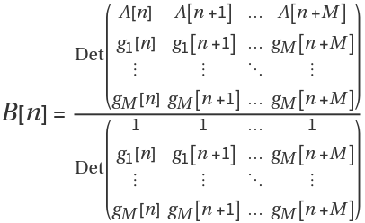
The Method "Cramer" calculates determinants:

In[6]:=

$bc = ResourceFunction["RichardsonExtrapolate"][1/( k - 1/2), {1/k, 1/k^2}, k, n, Method -> "Cramer"]$

Out[6]=

Use "LinearSolve":

In[7]:=

$bl = ResourceFunction["RichardsonExtrapolate"][1/( k - 1/2), {1/k, 1/k^2}, k, n, Method -> "LinearSolve"]$

Out[7]=

Compare the method outputs in a table:

In[8]:=

Out[8]=

They are all equivalent:

In[9]:=

Out[9]=

"BrezinskiE" is generally faster than the "LinearSolve" and "Cramer" methods for sequences and lists:

In[10]:=

(* Evaluate this cell to get the example input *) CloudGet["https://www.wolframcloud.com/obj/f6595b1c-8861-42eb-bcc0-32b9b5d135ba"]

Out[10]=

"BrezinskiE" and "LinearSolve" perform similarly on lists, while the "Cramer" Method is slower:

In[11]:=

(* Evaluate this cell to get the example input *) CloudGet["https://www.wolframcloud.com/obj/4ca3f3d7-af14-4624-ad11-6409f9c1cf36"]

Out[11]=

MinWorkingPrecision (2)

Set "MinWorkingPrecision", which applies SetPrecision on entries that have smaller Precision than the specified value:

In[12]:=

data1 = Table[1/(2 k + 1), {k, 1, 15}];
data2 = Table[1.`20/(2 k + 1), {k, 1, 15}];

In[13]:=

(* Evaluate this cell to get the example input *) CloudGet["https://www.wolframcloud.com/obj/1507b8cb-95d3-4d5d-993c-5777e2065628"]

Out[13]=

In numeric calculations, the "Cramer" Method preserves higher Precision:

In[14]:=

data1 = Table[1.`50/(2 k + 1), {k, 1, 30}];
data2 = Table[1/(2 k + 1), {k, 1, 30}];

In[15]:=

(* Evaluate this cell to get the example input *) CloudGet["https://www.wolframcloud.com/obj/19816bf2-ff3f-4c40-ae4e-38ac07c750e0"]

Out[15]=

In[16]:=

(* Evaluate this cell to get the example input *) CloudGet["https://www.wolframcloud.com/obj/1492ad4f-ba70-48e8-888a-9de81db7be9b"]

Out[16]=

Applications (6)

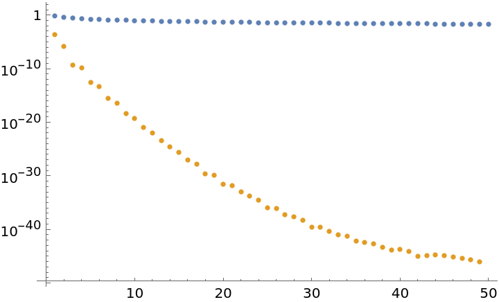
Calculate the convergence of the Basel series:

In[17]:=

$\!$ \*UnderoverscriptBox[\(\[Sum]$, $i = 1$, $\[Infinity]$] \*FractionBox[$1$, SuperscriptBox[$i$, $2$]]\)$

Out[17]=

Accelerate the convergence with RichardsonExtrapolate and plot a comparison:

In[18]:=

$partialsum = Table[\!$ \*UnderoverscriptBox[\(\[Sum]$, $i = 1$, $k$] \*FractionBox[$1$, SuperscriptBox[$i$, $2$]]\), {k, 1, 50}]; accsum = Table[ Last@ResourceFunction["RichardsonExtrapolate"][partialsum, n], {n, 1, 50 - 1}]; ListLogPlot[{Abs[partialsum - \[Pi]^2/6], Abs[accsum - \[Pi]^2/6]}, PlotRange -> All]$

Out[20]=

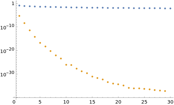
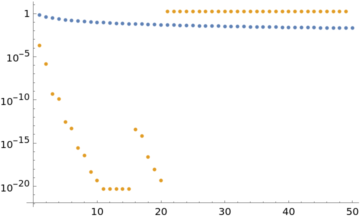
Calculate the convergence of the Leibniz formula for :

In[21]:=

$\!$ \*UnderoverscriptBox[\(\[Sum]$, $i = 0$, $\[Infinity]$]$ \*SuperscriptBox[\((\(-1$)\), $i$] \*FractionBox[$1$, $2 i + 1$]\)\)$

Out[21]=

Accelerate the convergence and plot a comparison:

In[22]:=

$partialsum = Table[\!$ \*UnderoverscriptBox[\(\[Sum]$, $i = 0$, $k$]$ \*SuperscriptBox[\((\(-1$)\), $i$] \*FractionBox[$1$, $2 i + 1$]\)\), {k, 1, 30}]; accsum = Table[ Last@ResourceFunction["RichardsonExtrapolate"][partialsum, Table[Table[1/k^i (-1)^k, {k, 1, 30}], {i, 1, n}]], {n, 1, 30 - 1}]; ListLogPlot[{Abs[partialsum - \[Pi]/4], Abs[accsum - \[Pi]/4]}, PlotRange -> All]$

Out[24]=

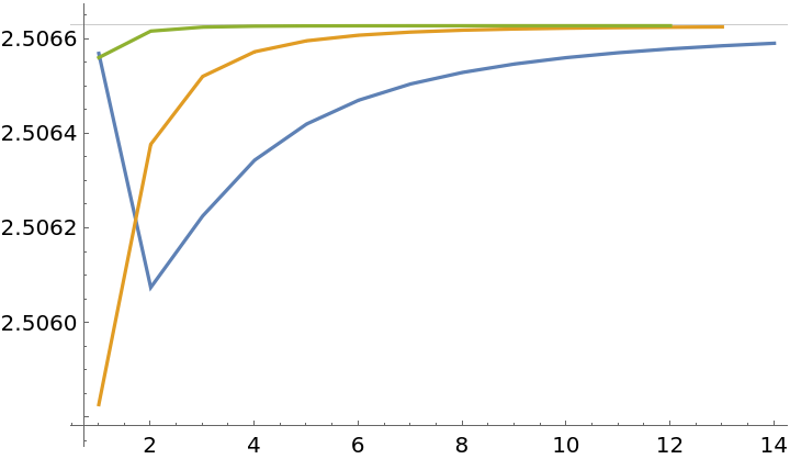
Calculate the convergence of Stirling's formula:

In[25]:=

$Limit[n!/(\[Sqrt]n n^n E^-n), n -> \[Infinity]]$

Out[25]=

Numerically verify the convergence using different orders:

In[26]:=

$ListLinePlot[ Table[ResourceFunction["RichardsonExtrapolate"][ Table[n!/(\[Sqrt]n n^n E^-n), {n, 1, 15}], M], {M, 1, 3}], PlotRange -> All, GridLines -> {{}, {Sqrt[2 \[Pi]]}}]$

Out[26]=

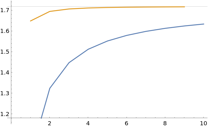
Numerically approximate the Zeta[1.2] function:

In[27]:=

$\!$ \*UnderoverscriptBox[\(\[Sum]$, $i = 1$, $\[Infinity]$] \*FractionBox[$1$, SuperscriptBox[$i$, $1.2`50$]]\)$

Out[27]=

Use RichardsonExtrapolate with different orders to attempt to accelerate the convergence:

In[28]:=

$partialsum = Table[\!$ \*UnderoverscriptBox[\(\[Sum]$, $i = 1$, $k$] \*FractionBox[$1$, SuperscriptBox[$i$, $1.2`20$]]\), {k, 1, 8}]; accsumlist = Table[ResourceFunction["RichardsonExtrapolate"][partialsum, Table[1/k^(0.2`20 + i), {i, 0, M - 1}, {k, 1, 8}]], {M, 1, 6}]; TableForm[accsumlist, TableHeadings -> {{"M=1", "M=2", "M=3", "M=4", "M=5", "M=6"}, {}}]$

Out[30]=

Plot a comparison when the sequence has more terms:

In[31]:=

$partialsum = Table[\!$ \*UnderoverscriptBox[\(\[Sum]$, $i = 1$, $k$] \*FractionBox[$1$, SuperscriptBox[$i$, $1.2`120$]]\), {k, 1, 50}]; accsum = Table[ ResourceFunction["RichardsonExtrapolate"][partialsum, Table[Table[1/k^(0.2`120 + i), {k, 1, 50}], {i, 0, M - 1}]] // Last, {M, 1, 50 - 1}]; ListLogPlot[Abs[accsum - Zeta[1.2`120]], PlotRange -> All]$

Out[33]=

Compute :

In[34]:=

In[35]:=

$\!$ \*SubsuperscriptBox[\(\[Integral]$, $0$, $1$]$f[ x] \[DifferentialD]x$\)$

Out[35]=

Accelerate a (left) Riemann sum approximating :

In[36]:=

In[37]:=

Out[37]=

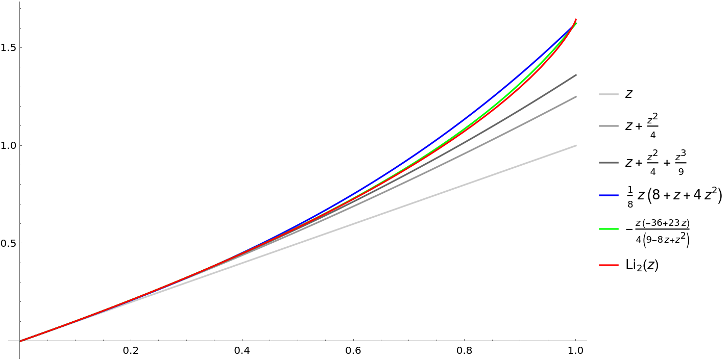
Approximate the PolyLog[2,z] function from only 3 terms in its Taylor expansion:

In[38]:=

$taylorpoly = Table[\!$ \*UnderoverscriptBox[\(\[Sum]$, $i = 1$, $k$]$ \*FractionBox[\(1$, SuperscriptBox[$i$, $2$]] \*SuperscriptBox[$z$, $i$]\)\), {k, 1, 3}];$

In[39]:=

Out[39]=

Use an auxiliary sequence:

In[40]:=

$accpoly2 = ResourceFunction["RichardsonExtrapolate"][taylorpoly, Table[Table[1/k^i z^k, {k, 1, 3}], {i, 1, 2}]] // Simplify$

Out[40]=

Compare the approximations with the original function in a plot:

In[41]:=

Plot[{taylorpoly, accpoly, accpoly2, PolyLog[2, z]}, {z, 0, 1},
PlotStyle -> {GrayLevel[0.8], GrayLevel[0.6], GrayLevel[0.4], Blue, Green, Red},
PlotLegends -> "Expressions",
ImageSize -> Large]

Out[41]=

Properties and Relations (5)

RichardsonExtrapolate is linear:

In[42]:=

$ResourceFunction[ "RichardsonExtrapolate"][\[Alpha] a[k] + \[Beta] b[k], 1, k, n] == \[Alpha] ResourceFunction["RichardsonExtrapolate"][a[k], 1, k, n] + \[Beta] ResourceFunction["RichardsonExtrapolate"][b[k], 1, k, n]$

Out[42]=

In[43]:=

Out[43]=

RichardsonExtrapolate reduces the length of a List:

In[44]:=

length = 10;
M = 3;
ResourceFunction["RichardsonExtrapolate"][
Table[1/(2 k + 1), {k, 1, length}], M]

Out[46]=

In[47]:=

Out[47]=

If a sequence a[k] is convergent, then a[k] and its transformed version both converge to the same limit:

In[48]:=

In[49]:=

$Limit[{a[n], ResourceFunction["RichardsonExtrapolate"][a[k], 1, k, n]}, n -> \[Infinity]]$

Out[78]=

RichardsonExtrapolate can accelerate the convergence of logarithmic sequences:

In[79]:=

$a[k_] := Sqrt[k + k^2] - k Limit[a[k], k -> \[Infinity]]$

Out[80]=

In[81]:=

$Limit[(ResourceFunction["RichardsonExtrapolate"][a[k], 1, k, k] - 1/2)/(a[k] - 1/2), k -> \[Infinity]]$

Out[81]=

RichardsonExtrapolate can eliminate series coefficients from the asymptotic expansion of a sequence:

In[82]:=

$Series[1/(2 k + 1), {k, \[Infinity], 3}]$

Out[82]=

In[83]:=

$Series[ResourceFunction["RichardsonExtrapolate"][1/(2 k + 1), 1, k, k], {k, \[Infinity], 3}]$

Out[83]=

Possible Issues (2)

A failure to find the appropriate auxiliary sequence can cause divergent behavior:

In[84]:=

$partialsum = Table[\!$ \*UnderoverscriptBox[\(\[Sum]$, $i = 0$, $k$]$ \*SuperscriptBox[\((\(-1$)\), $i$] \*FractionBox[$1$, $2\ i + 1$]\)\), {k, 1, 10}] // N$

Out[84]=

In[85]:=

Out[85]=

Use an appropriate auxiliary sequence:

In[86]:=

$ResourceFunction["RichardsonExtrapolate"][partialsum, Table[Table[(-1)^k 1/k^i, {k, 1, 10}], {i, 1, 4}]] // N$

Out[86]=

Numeric errors can have a dramatic effect on the results:

In[87]:=

$partialsum = N[Table[\!$ \*UnderoverscriptBox[\(\[Sum]$, $i = 1$, $k$] \*FractionBox[$1$, SuperscriptBox[$i$, $2$]]\), {k, 1, 50}], 20]; accsum = Table[ Last@ResourceFunction["RichardsonExtrapolate"][partialsum, n], {n, 1, 50 - 1}]; ListLogPlot[{Abs[partialsum - \[Pi]^2/6], Abs[SetPrecision[accsum, 50] - \[Pi]^2/6]}, PlotRange -> All]$

Out[88]=

Neat Examples (2)

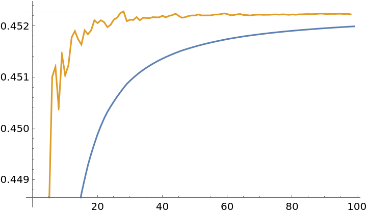
Consider the PrimeZetaP[2] partial sums:

In[89]:=

$\!$ \*UnderoverscriptBox[\(\[Sum]$, $k = 1$, $\[Infinity]$] \*FractionBox[$1$, SuperscriptBox[$Prime[k]$, $2$]]\)$

Out[89]=

In[90]:=

Out[90]=

Approximate with RichardsonExtrapolate and compare the results:

In[91]:=

$partialsum = Table[Sum[1/Prime[k]^2, {k, 1, n}], {n, 2, 100}]; accsum = ResourceFunction["RichardsonExtrapolate"][ partialsum, {Table[1/(k Log[k]^2), {k, 2, 100}]}]; ListLinePlot[{partialsum, accsum}, GridLines -> {{}, {PrimeZetaP[2]}}]$

Out[92]=

Compare the limits in a table:

In[93]:=

$TableForm[{PrimeZetaP[2], partialsum // Last, accsum // Last} // N, TableHeadings -> {{"P(2)", "\!$\*SuperscriptBox[\(100$, $th$]\) partial sum of \!$\*FractionBox[\(1$, SuperscriptBox[SubscriptBox[$p$, $k$], $2$]]\)", "Richardson Estrapolation"}}]$

Out[93]=

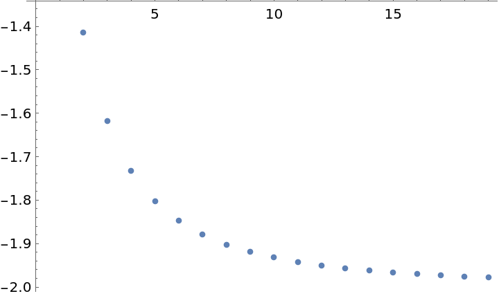
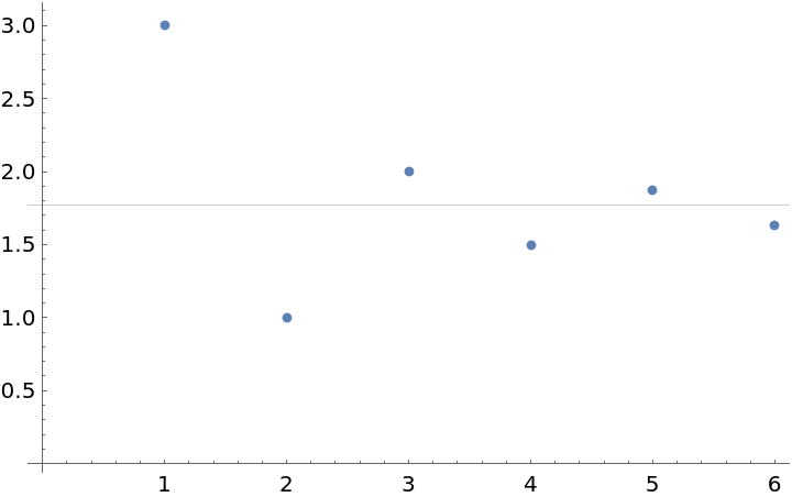
Approximate the Eigenvalues of an operator by a sequence of truncated matrix representations:

In[94]:=

$h[n_] := SparseArray[{Band[{2, 1}] -> 1, Band[{1, 2}] -> 1}, {n, n}] MatrixForm[h[5]]$

Out[95]=

In[96]:=

Out[97]=

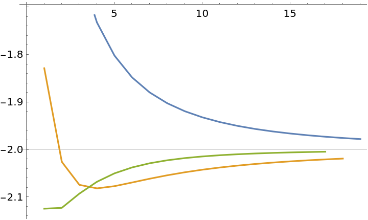
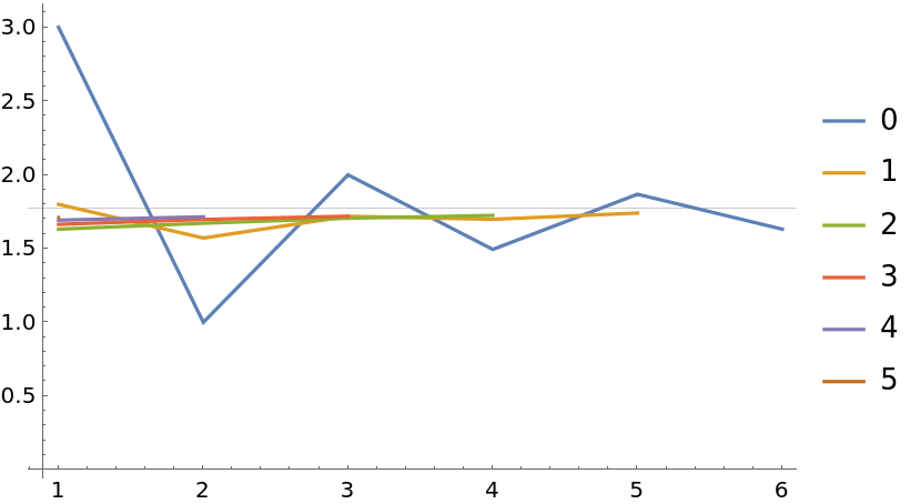
Accelerate the convergence using RichardsonExtrapolate:

In[98]:=

Out[98]=

Approximating the ground state of the antiferromagnetic Heisenberg spin chain (4)

Construct the Hamiltonian of the model, which is a 2ⁿ×2ⁿ dimensional matrix, where n is the length of the spin chain:

In[99]:=

$S[a_][j_][n_] := KroneckerProduct @@ Table[If[i == j, PauliMatrix[a], IdentityMatrix[2]], {i, 1, n}] H[n_] := -Sum[ Sum[S[a][j][n] . S[a][Mod[j + 1 - 1, n] + 1][n], {a, 1, 3}], {j, 1, n}]$

Calculate the ground state energy density by exact diagonalization:

In[100]:=

nMax = 7;
ListPlot[eList = Table[(Eigenvalues[N[H[n]]] // Sort // Last)/n, {n, 2, nMax}], GridLines -> {{}, {-1 + 4 Log[2]}}]

Out[101]=

Use Richardson Extrapolation to estimate the thermodynamic limit as n→∞:

In[102]:=

$MMax = 5; ListLinePlot[ Table[ResourceFunction["RichardsonExtrapolate"][eList, Evaluate[Table[Table[(-1)^n/n^i, {n, 2, nMax}], {i, 1, M}]]], {M, 0, MMax}], GridLines -> {{}, {-1 + 4 Log[2]}}, PlotRange -> All, PlotLegends -> Range[0, 5]]$

Out[103]=

In[104]:=

$TableForm[ Table[ResourceFunction["RichardsonExtrapolate"][eList, Evaluate[Table[Table[(-1)^n/n^i, {n, 2, nMax}], {i, 1, M}]]], {M, 0, MMax}], TableHeadings -> {{"M=0", "M=1", "M=2", "M=3", "M=4", "M=5"}, {"n=2", "n=3", "n=4", "n=5", "n=6", "n=7"}}]$

Out[104]=

Compare the results with the exact ground state:

In[105]:=

Out[105]=

In[106]:=

$TableForm[ Table[Abs[# - eExact] & /@ ResourceFunction["RichardsonExtrapolate"][eList, Evaluate[Table[Table[(-1)^n/n^i, {n, 2, nMax}], {i, 1, M}]]], {M, 0, MMax}], TableHeadings -> {{"M=0", "M=1", "M=2", "M=3", "M=4", "M=5"}, {"n=2", "n=3", "n=4", "n=5", "n=6", "n=7"}}]$

Out[106]=

Publisher

Jozsef Konczer

Version History

1.0.0 – 28 January 2021

Source Metadata

Citation:
- Bender, C., Orszag, S, Advanced mathematical methods for scientists and engineers. New York: Springer, 1999.
- Osada, N., "Acceleration methods for slowly convergent sequences and their applications." Ph.D. thesis, Nagoya University, Japan, 1993.
- Brezinski, C., "Convergence Acceleration During the 20th Century." Journal of Computational and Applied Mathematics, 122, 1-21, 2000.
- Brezinski, C., Zaglia, M. R., Extrapolation methods: Volume 2: Theory and practice. Oxford, England: North-Holland, 1991.

Related Resources

License Information

This work is licensed under a Creative Commons Attribution 4.0 International License