Wolfram Function Repository
Instant-use add-on functions for the Wolfram Language
Function Repository Resource:
Visualize the recurrence of a single discrete time series on a lattice
ResourceFunction["RecurrencePlot"][ts] shows the recurrence plot of the time series ts. | |
ResourceFunction["RecurrencePlot"][{ts1,ts2}] shows the recurrence plot for a pair of time series. |
 where
where  is a unit step, ε is a threshold, where
  is a norm, and
  are each elements of the time series vectors.
| "RecurrenceThreshold" | 1 | value of threshold ε used |
| "RecurrenceType" | "Standard" | type of recurrence |
is taken to be the Identity function.Recurrence plot of list of random integers:
| In[1]:= | ![ResourceFunction["RecurrencePlot"][RandomInteger[10, 30]]](https://www.wolframcloud.com/obj/resourcesystem/images/d35/d35fa3e8-aaed-47d0-b2ac-2a77bdd2f9ac/48a4bbd0ddc75787.png) |
| Out[1]= | 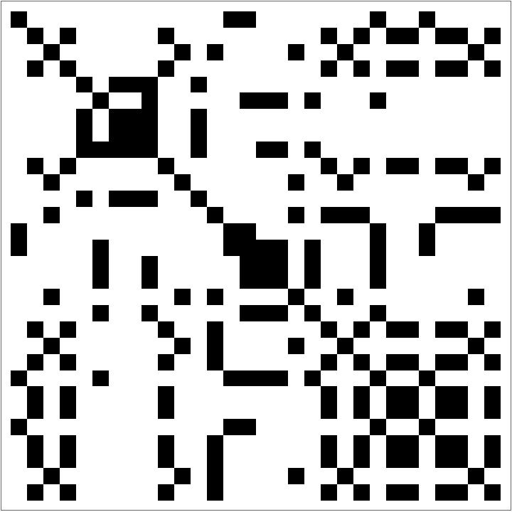 |
Recurrence plot of a one-dimensional list of ordered integers:
| In[2]:= | ![ResourceFunction["RecurrencePlot"][Range[10, 30], Frame -> None, ColorFunction -> "Rainbow"]](https://www.wolframcloud.com/obj/resourcesystem/images/d35/d35fa3e8-aaed-47d0-b2ac-2a77bdd2f9ac/45dfe417d594b002.png) |
| Out[2]= |  |
Recurrence plot of discrete data from a sine function:
| In[3]:= | ![ResourceFunction["RecurrencePlot"][Table[Sin[x], {x, 0, 10, .1}]]](https://www.wolframcloud.com/obj/resourcesystem/images/d35/d35fa3e8-aaed-47d0-b2ac-2a77bdd2f9ac/30439932b75b2b7d.png) |
| Out[3]= |  |
Recurrence plot of a trigonometric operation:
| In[4]:= | ![ResourceFunction["RecurrencePlot"][
Table[Sin[x]*Cos[y], {x, -10, 10, 1}, {y, -10, 10, 1}]]](https://www.wolframcloud.com/obj/resourcesystem/images/d35/d35fa3e8-aaed-47d0-b2ac-2a77bdd2f9ac/5a17939a018eef54.png) |
| Out[4]= | 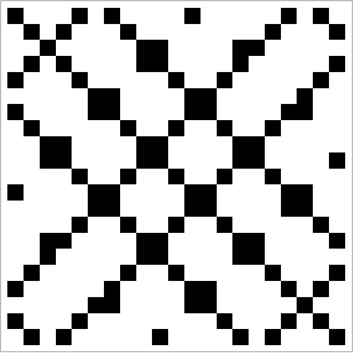 |
Recurrence plot of random and range discrete lists:
| In[5]:= | ![ResourceFunction[
"RecurrencePlot"][{RandomInteger[10, 100], Range[100]}, "RecurrenceType" -> "Global" , ColorFunction -> GrayLevel, Frame -> None]](https://www.wolframcloud.com/obj/resourcesystem/images/d35/d35fa3e8-aaed-47d0-b2ac-2a77bdd2f9ac/441378b8b3837bb1.png) |
| Out[5]= |  |
Cross-recurrence plot from two random discrete lists:
| In[6]:= | ![ResourceFunction[
"RecurrencePlot"][{RandomInteger[10, 100], RandomInteger[10, 100]}, ColorRules -> {0 -> Yellow, 1 -> Orange}, Frame -> None]](https://www.wolframcloud.com/obj/resourcesystem/images/d35/d35fa3e8-aaed-47d0-b2ac-2a77bdd2f9ac/0837f1ea75919258.png) |
| Out[6]= | 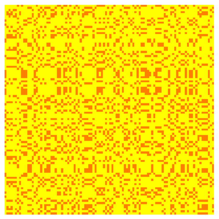 |
Cross-recurrence plot of two trigonometric functions:
| In[7]:= | ![ResourceFunction[
"RecurrencePlot"][{Table[Sin[x], {x, 0, 100, .5}], Table[Tan[x], {x, 0, 100, .5}]}]](https://www.wolframcloud.com/obj/resourcesystem/images/d35/d35fa3e8-aaed-47d0-b2ac-2a77bdd2f9ac/3914b6a99fdff483.png) |
| Out[7]= | 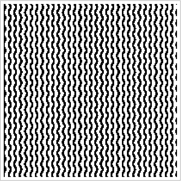 |
Global cross-recurrence plot of two random lists:
| In[8]:= | ![ResourceFunction[
"RecurrencePlot"][{RandomInteger[10, 100], RandomInteger[10, 100]}, "RecurrenceType" -> "Global", ColorFunction -> Hue, Frame -> None]](https://www.wolframcloud.com/obj/resourcesystem/images/d35/d35fa3e8-aaed-47d0-b2ac-2a77bdd2f9ac/6d01b568b5efed57.png) |
| Out[8]= | 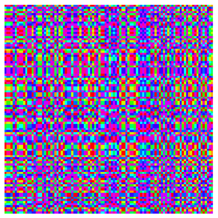 |
Global recurrence plot of elementary cellular automata rules:
| In[10]:= | ![Manipulate[
ca = CellularAutomaton[rule, RandomInteger[1, 100], 100];
GraphicsGrid[{{ArrayPlot[ca, Frame -> None],
ResourceFunction["RecurrencePlot"][Total[Transpose[ca]], "RecurrenceType" -> "Global", ColorFunction -> Hue, Frame -> None]}}],
{{rule, 110}, 0, 255, 1}, SaveDefinitions -> True]](https://www.wolframcloud.com/obj/resourcesystem/images/d35/d35fa3e8-aaed-47d0-b2ac-2a77bdd2f9ac/69a51bd32d34a1ef.png) |
| Out[10]= | 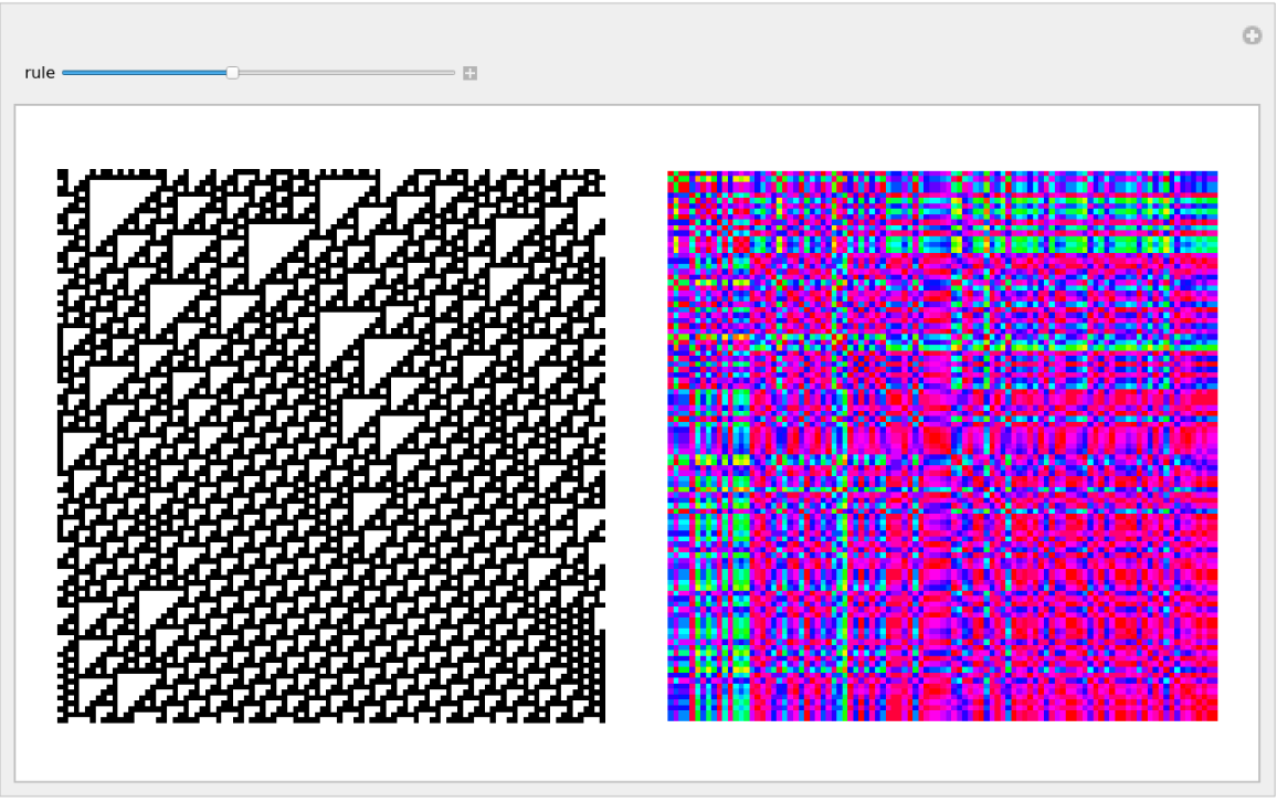 |
Visualize Bitcoin data:
| In[11]:= | ![Take[Flatten[
ToCharacterCode[
BlockchainBlockData[300000, "TransactionList", BlockchainBase -> "Bitcoin"]]] - 60, 100]](https://www.wolframcloud.com/obj/resourcesystem/images/d35/d35fa3e8-aaed-47d0-b2ac-2a77bdd2f9ac/16c0fc898fe6a2b5.png) |
| Out[11]= |  |
| In[12]:= | ![ResourceFunction["RecurrencePlot"][%]](https://www.wolframcloud.com/obj/resourcesystem/images/d35/d35fa3e8-aaed-47d0-b2ac-2a77bdd2f9ac/3b0d1c2972e6974e.png) |
| Out[12]= | 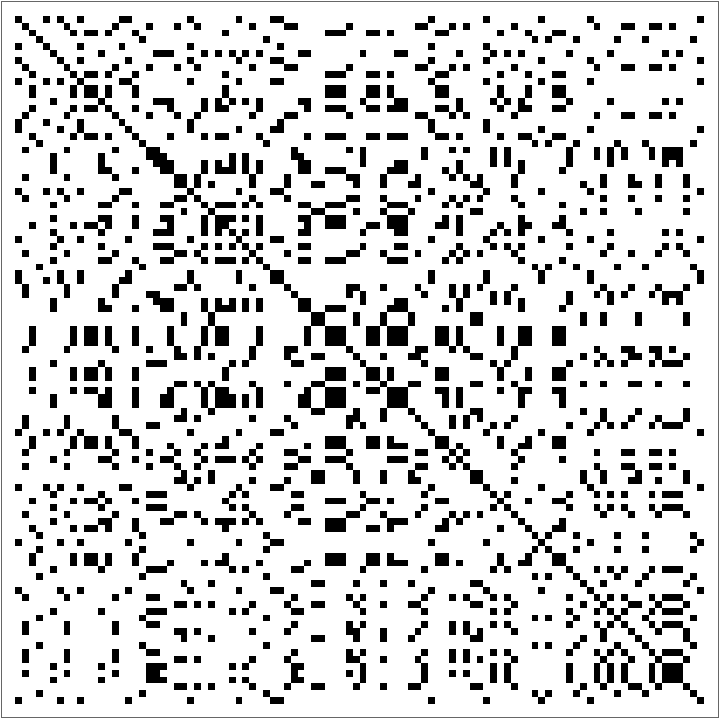 |
Dynamic visualization of a cross-recurrence plot of trigonometric functions:
| In[13]:= | ![Manipulate[ResourceFunction["RecurrencePlot"][
{Table[Sin[x fx],
{x, -10, 10, 1}],
Table[Cos[y fy],
{y, -10, 10, 1}]}],
{{fx, 6}, 1, 10},
{{fy, 5}, 1, 10}, SaveDefinitions -> True]](https://www.wolframcloud.com/obj/resourcesystem/images/d35/d35fa3e8-aaed-47d0-b2ac-2a77bdd2f9ac/01170bc0928adbce.png) |
| Out[13]= | 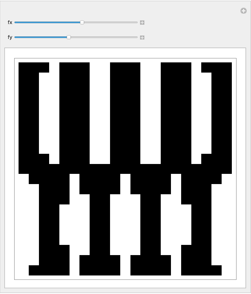 |
Wolfram Language 13.0 (December 2021) or above
This work is licensed under a Creative Commons Attribution 4.0 International License
![ResourceFunction["RecurrencePlot"][RandomInteger[7, 100], Frame -> None]](https://www.wolframcloud.com/obj/resourcesystem/images/d35/d35fa3e8-aaed-47d0-b2ac-2a77bdd2f9ac/50ad1a89322d693b.png)