Wolfram Function Repository
Instant-use add-on functions for the Wolfram Language
Function Repository Resource:
Compute quantile regression fits over a time series, a list of numbers or a list of numeric pairs
ResourceFunction["QuantileRegression"][data,knots,probs] does quantile regression over the times series or data array data using the knots specification knots for the probabilities probs. | |
ResourceFunction["QuantileRegression"][data,knots,probs,opts] does quantile regression with the options opts. |
| InterpolationOrder | 3 | interpolation order |
| Method | LinearProgramming | method for the quantile regression computations |
Make a random signal:
| In[1]:= | ![SeedRandom[23];
n = 200;
randData = Transpose[{Range[n], RandomReal[{0, 100.}, n]}];](https://www.wolframcloud.com/obj/resourcesystem/images/5a6/5a6171c2-336f-4f2f-ad62-2baf3098c6b7/3d896d280c3b7ac0.png) |
Compute QuantileRegression with five knots for the probabilities 0.25 and 0.75:
| In[2]:= |
Here are the formulas of the obtained regression quantiles:
| In[3]:= |
| Out[3]= |  |
Here is a plot of the original data and the obtained regression quantiles:
| In[4]:= |
| Out[4]= | 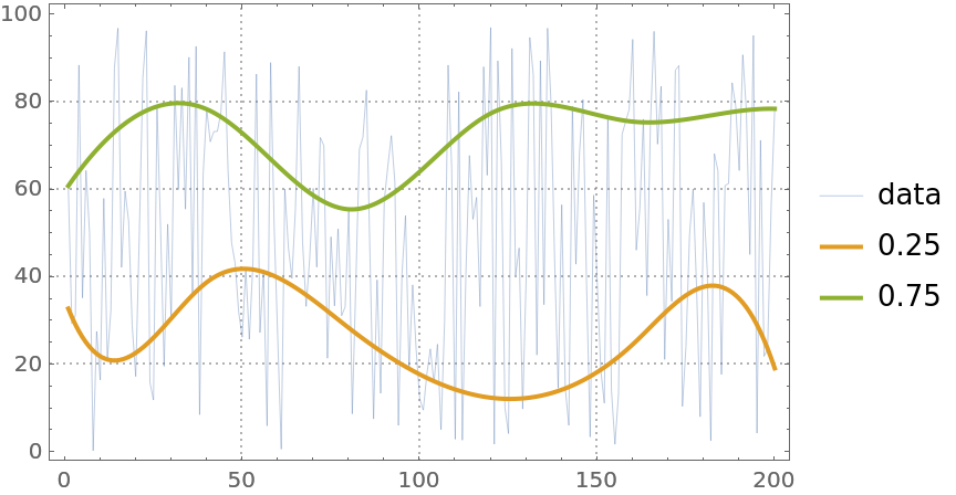 |
Find the fraction of the data points that are under the second regression quantile:
| In[5]:= |
| Out[5]= |
The obtained fraction is close to the second probability, 0.75, given to QuantileRegression.
Here is a quantile regression computation over a numerical vector:
| In[6]:= | ![vecData = Sin[Range[200]/6] + RandomReal[{-0.5, 0.5}, 200];
qFunc = First@ResourceFunction["QuantileRegression"][vecData, 12, 0.5];
ListLinePlot[{vecData, qFunc[#] & /@ Range[Length[vecData]]}, PlotRange -> All, PlotTheme -> "Detailed", PlotLegends -> {"vector", "fit"}]](https://www.wolframcloud.com/obj/resourcesystem/images/5a6/5a6171c2-336f-4f2f-ad62-2baf3098c6b7/7e2299b2f6a99555.png) |
| Out[6]= | 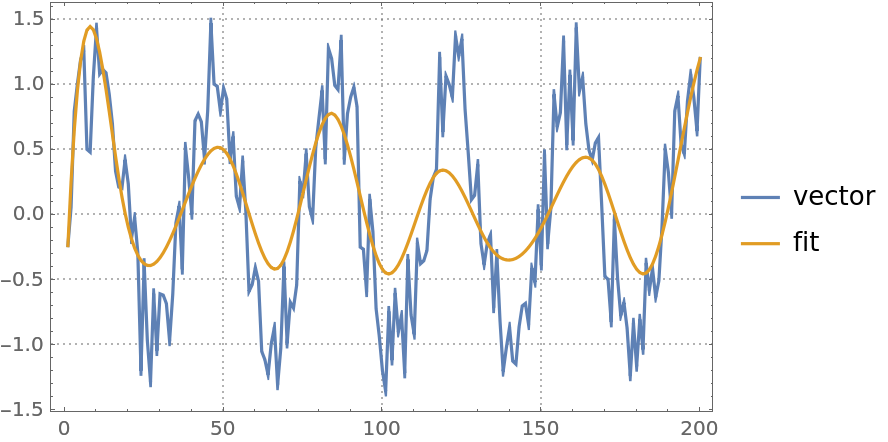 |
Here is a quantile regression computation over a time series object:
| In[7]:= | ![finData = FinancialData["GE", {{2010, 1, 1}, {2019, 10, 15}, "Week"}];
qFunc = First@ResourceFunction["QuantileRegression"][finData, 12, 0.5];
DateListPlot[{finData, {#, qFunc[#]} & /@ finData["Times"]}, Joined -> {False, True}, PlotLegends -> {"time series", "fit"}]](https://www.wolframcloud.com/obj/resourcesystem/images/5a6/5a6171c2-336f-4f2f-ad62-2baf3098c6b7/66789d5517ad15dd.png) |
| Out[7]= | 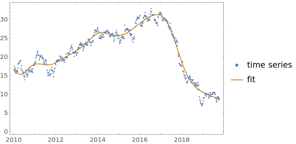 |
The second argument—the knots specification—can be an integer specifying the number of knots or a list of numbers specifying the knots of the B-spline basis:
| In[8]:= |
The option InterpolationOrder specifies the polynomial order of the B-spline basis. Its values are expected to be non-negative integers:
| In[9]:= | ![qFuncs = Table[First@
ResourceFunction["QuantileRegression"][randData, 5, 0.5, InterpolationOrder -> i], {i, {0, 1, 3}}];](https://www.wolframcloud.com/obj/resourcesystem/images/5a6/5a6171c2-336f-4f2f-ad62-2baf3098c6b7/18455789da812f8a.png) |
| In[10]:= | ![ListLinePlot[
Prepend[(#1 /@ Range[Length[randData]] &) /@ qFuncs, randData], PlotStyle -> {Thin, Thick, Thick, Thick}, PlotLegends -> Prepend[{"0.5, interpolation order 0", "0.5, interpolation order 1",
"0.5, interpolation order 3"}, "data"], PlotTheme -> "Detailed"]](https://www.wolframcloud.com/obj/resourcesystem/images/5a6/5a6171c2-336f-4f2f-ad62-2baf3098c6b7/225c262cbe3aacd3.png) |
| Out[10]= | 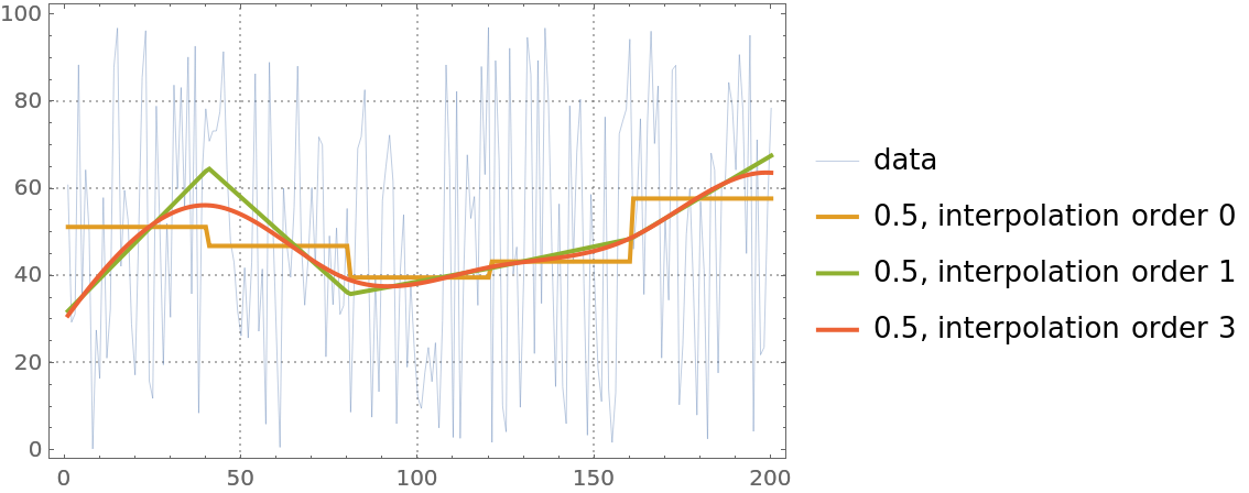 |
QuantileRegression uses LinearProgramming. Additional parameters can be passed to LinearProgramming with the Method option:
| In[11]:= |
| In[12]:= |
| Out[12]= | 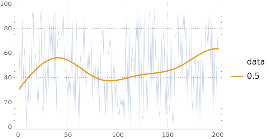 |
Here is heteroscedastic data (the variance is not constant with respect to the predictor variable):
| In[13]:= | ![distData = Table[{x, Exp[-x^2] + RandomVariate[
NormalDistribution[0, .15 \[Sqrt](Abs[1.5 - x]/1.5)]]}, {x, -3, 3, .01}];
ListPlot[distData, PlotTheme -> "Detailed", ImageSize -> Medium]](https://www.wolframcloud.com/obj/resourcesystem/images/5a6/5a6171c2-336f-4f2f-ad62-2baf3098c6b7/7c6838564deadc3a.png) |
| Out[13]= | 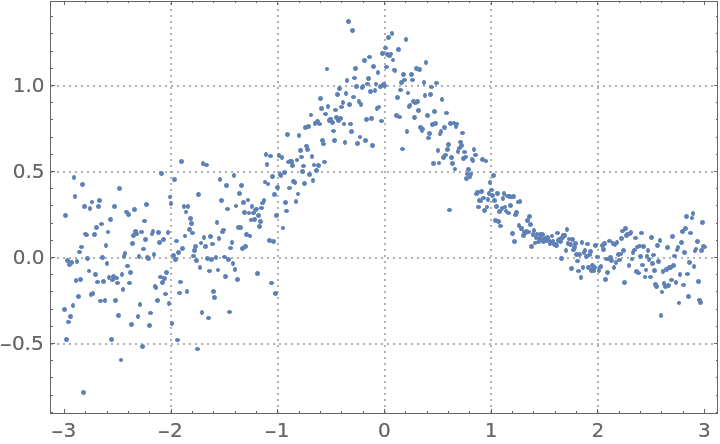 |
Find quantile regression fits:
| In[14]:= |
Plot the data and the regression quantiles:
| In[15]:= | ![ListPlot[
Prepend[(Transpose[{distData[[All, 1]], #1 /@ distData[[All, 1]]}] &) /@ qFuncs, distData], Joined -> Prepend[Table[True, Length[probs]], False], PlotLegends -> Prepend[probs, "data"], PlotTheme -> "Detailed", FrameLabel -> {"Time", "Temperature"}, ImageSize -> Medium]](https://www.wolframcloud.com/obj/resourcesystem/images/5a6/5a6171c2-336f-4f2f-ad62-2baf3098c6b7/4fb68f74ec21b0c2.png) |
| Out[15]= | 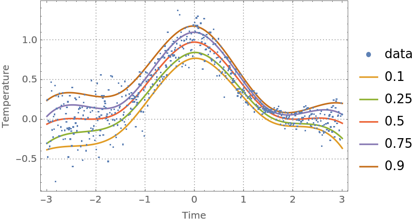 |
Note that the regression quantiles clearly outline the heteroscedastic nature of the data.
A certain contextual type of anomaly is a subset of points that have variance very different than other subsets. Using quantile regression we can (1) evaluate the regressor-dependent variance for each point using the regression quantiles 0.25 and 0.75; and (2) find the points that have outlier variances.
Here we compute and plot the variance estimates for a signal:
| In[16]:= | ![qFuncs = ResourceFunction["QuantileRegression"][distData, 4, {0.25, 0.75}];
variances = Map[Abs@*Subtract @@ Through[qFuncs[#]] &, distData[[All, 1]]];
ListPlot[variances, PlotRange -> All]](https://www.wolframcloud.com/obj/resourcesystem/images/5a6/5a6171c2-336f-4f2f-ad62-2baf3098c6b7/5f40fb09440e97f0.png) |
| Out[16]= | 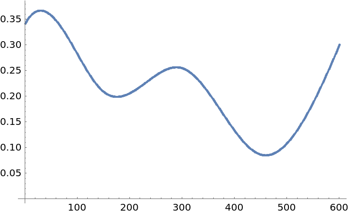 |
Find the lower and upper thresholds for the variance outliers:
| In[17]:= |
| Out[17]= |
Find the outlier positions:
| In[18]:= |
Plot the data and the outliers found:
| In[19]:= | ![ListPlot[{distData, distData[[varianceOutlierPositions]]}, PlotRange -> All, PlotLegends -> {"data", "variance outliers"}]](https://www.wolframcloud.com/obj/resourcesystem/images/5a6/5a6171c2-336f-4f2f-ad62-2baf3098c6b7/147b95b6fa072707.png) |
| Out[19]= | 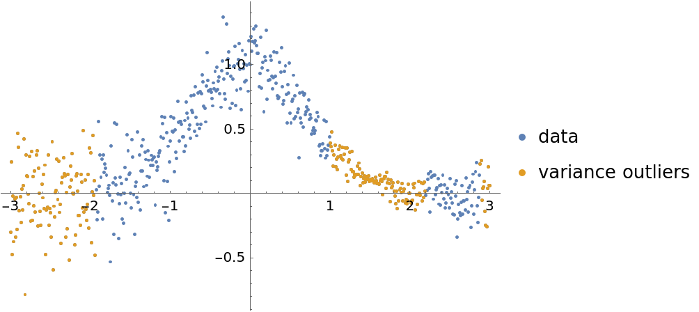 |
Here is a financial time series:
| In[20]:= |
| Out[20]= |
| In[21]:= |
| Out[21]= |
Do a quantile regression fit and plot it:
| In[22]:= | ![qFunc = First@ResourceFunction["QuantileRegression"][finData, 50, 0.5];
DateListPlot[{finData, {#, qFunc[#]} & /@ finData["Times"]}, PlotTheme -> "Detailed", AspectRatio -> 1/4, ImageSize -> Large, PlotLegends -> {"data", "fit"}]](https://www.wolframcloud.com/obj/resourcesystem/images/5a6/5a6171c2-336f-4f2f-ad62-2baf3098c6b7/47df7f4e50bed494.png) |
| Out[22]= | 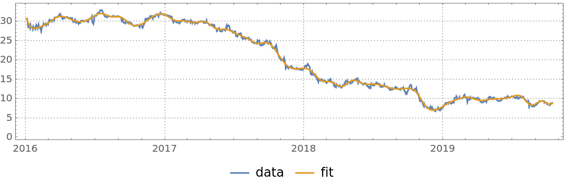 |
Here are the errors of the fit found:
| In[23]:= | ![DateListPlot[
Map[{#[[1]], (qFunc[#[[1]]] - #[[2]])/#[[2]]} &, QuantityMagnitude[finData["Path"]]], Joined -> False, PlotRange -> All, Filling -> Axis, PlotTheme -> "Detailed", AspectRatio -> 1/4, ImageSize -> Large]](https://www.wolframcloud.com/obj/resourcesystem/images/5a6/5a6171c2-336f-4f2f-ad62-2baf3098c6b7/4db88f3e7fad4902.png) |
| Out[23]= | 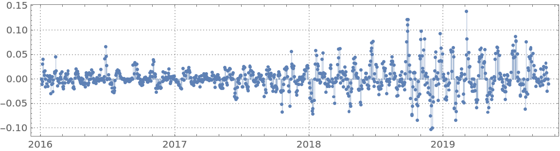 |
Find anomalies' positions in the list of fit errors:
| In[24]:= |
| Out[24]= |
Plot the data, fit and anomalies:
| In[25]:= | ![DateListPlot[{finData, {#, qFunc[#]} & /@ finData["Times"], finData["Path"][[pos]]}, PlotTheme -> "Detailed", AspectRatio -> 1/4, ImageSize -> Large, Joined -> {False, True, False}, PlotStyle -> {{GrayLevel[0.5`], Opacity[0.5`]}, {Red, Thick}, {Blue, PointSize[0.01`]}}, PlotLegends -> {"data", "fit", "anomalies"}]](https://www.wolframcloud.com/obj/resourcesystem/images/5a6/5a6171c2-336f-4f2f-ad62-2baf3098c6b7/059472f24bee9775.png) |
| Out[25]= | 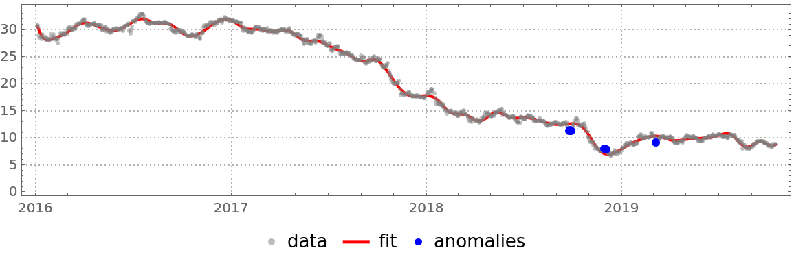 |
Get temperature data:
| In[26]:= |
| Out[26]= |
Convert the time series into a list of numeric pairs:
| In[27]:= |
Compute quantile regression fits:
| In[28]:= |
Plot the data and the regression quantiles:
| In[29]:= | ![DateListPlot[
Prepend[(Transpose[{tempData[[All, 1]], #1 /@ tempData[[All, 1]]}] &) /@ qFuncs, tempData], Joined -> Prepend[Table[True, Length[probs]], False], PlotLegends -> Prepend[probs, "temperature data"], AspectRatio -> 1/4, PlotTheme -> "Detailed", FrameLabel -> {"Time", "Temperature"}, ImageSize -> Large]](https://www.wolframcloud.com/obj/resourcesystem/images/5a6/5a6171c2-336f-4f2f-ad62-2baf3098c6b7/401924979c5f2ceb.png) |
| Out[29]= |  |
Find an estimate of the conditional cumulative distribution function (CDF) at the date 2017-10-01:
| In[30]:= |
| Out[30]= | 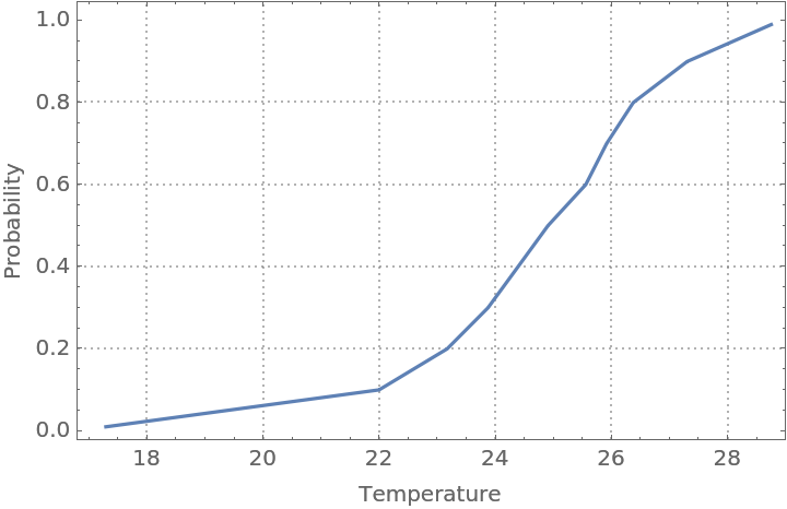 |
Find outliers in the temperature data—outliers are defined as points below or above the 0.02 and 0.98 regression quantiles respectively:
| In[31]:= |
| In[32]:= |
| In[33]:= | ![DateListPlot[{tempData, {#, qFuncs[[1]][#]} & /@ tempData[[All, 1]], {#, qFuncs[[-1]][#]} & /@ tempData[[All, 1]], bottomOutliers, topOutliers}, Sequence[
PlotTheme -> "Detailed", PlotLegends -> {"original data", "bottom regression quantile", "top regression quantile", "bottom outliers", "top outliers"}, Joined -> {False, True, True, False, False}, PlotStyle -> {{Gray,
PointSize[0.002]}, {Black, Thin}, {Black, Thin}, {
PointSize[0.012]}, {
PointSize[0.012]}}, AspectRatio -> 1/4, FrameLabel -> {"Time", "Temperature"}, ImageSize -> Large]]](https://www.wolframcloud.com/obj/resourcesystem/images/5a6/5a6171c2-336f-4f2f-ad62-2baf3098c6b7/6265be3427f0d33e.png) |
| Out[33]= | 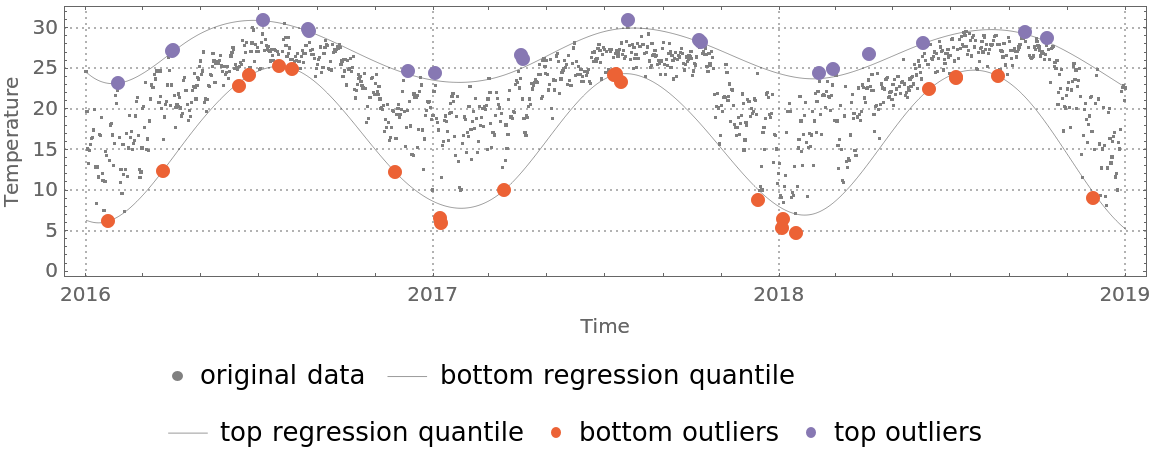 |
QuantileRegression can be compared with FindFormula, Fit, LinearModelFit and NonlinearModelFit:
| In[34]:= |
| In[35]:= |
| In[36]:= | ![ListLinePlot[{distData, {#, qFunc[#]} & /@ distData[[All, 1]], {#, fFunc[#]} & /@ distData[[All, 1]]}, PlotStyle -> {Thin, Thick, Thick}, PlotLegends -> {"data", 0.5`, "mean"}, PlotTheme -> "Detailed"]](https://www.wolframcloud.com/obj/resourcesystem/images/5a6/5a6171c2-336f-4f2f-ad62-2baf3098c6b7/6148429ebba9e5fd.png) |
| Out[36]= |  |
Quantile regression is much more robust than linear regression. In order to demonstrate that, add a few large outliers in the data:
| In[37]:= |
Here quantile regression and linear regression are applied, as in the previous example:
| In[38]:= |
| In[39]:= |
Here is a plot of the obtained curves. Note that the curve corresponding to linear regression is different and a worse fit than the one from the previous example:
| In[40]:= | ![ListLinePlot[{distData3, {#, qFunc[#]} & /@ distData3[[All, 1]], {#, fFunc[#]} & /@ distData3[[All, 1]]}, PlotStyle -> {Thin, Thick, Thick}, PlotLegends -> {"data", 0.5`, "mean"}, PlotTheme -> "Detailed"]](https://www.wolframcloud.com/obj/resourcesystem/images/5a6/5a6171c2-336f-4f2f-ad62-2baf3098c6b7/7597a8353ba71c72.png) |
| Out[40]= | 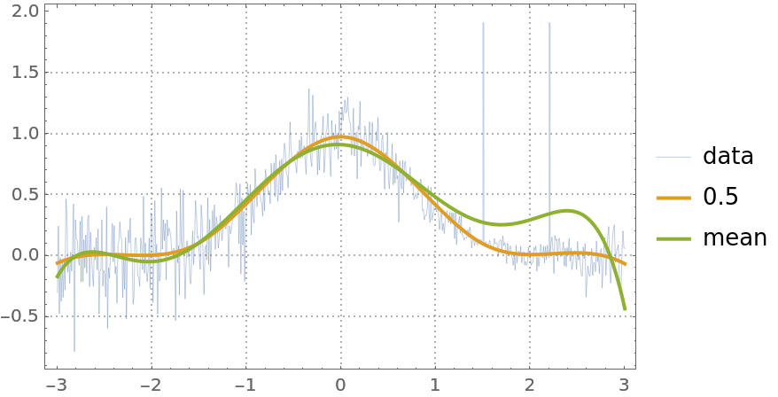 |
Because of the linear programming formulation for some data and knots specifications, the computations can be slow.
For most data, the quantile regression fitting for probabilities 0 and 1 produces regression quantiles that are "too far away from the data."
Find regression quantiles for probabilities 0 and 0.5 and plot them:
| In[41]:= | ![probs = {0, 0.5};
qFuncs = ResourceFunction["QuantileRegression"][distData, 6, probs];
ListPlot[
Prepend[(Transpose[{distData[[All, 1]], #1 /@ distData[[All, 1]]}] &) /@ qFuncs, distData], Joined -> Prepend[Table[True, Length[probs]], False], PlotLegends -> Prepend[probs, "data"], PlotTheme -> "Detailed", FrameLabel -> {"Time", "Temperature"}, ImageSize -> Medium]](https://www.wolframcloud.com/obj/resourcesystem/images/5a6/5a6171c2-336f-4f2f-ad62-2baf3098c6b7/7af13d69971f5171.png) |
| Out[41]= | 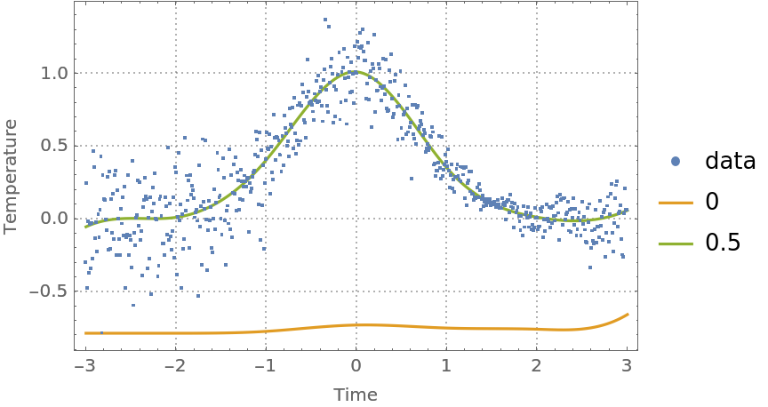 |
Find regression quantiles for probabilities 0.5 and 1 and plot them:
| In[42]:= | ![probs = {0.5, 1};
qFuncs = ResourceFunction["QuantileRegression"][distData, 6, probs];
ListPlot[
Prepend[(Transpose[{distData[[All, 1]], #1 /@ distData[[All, 1]]}] &) /@ qFuncs, distData], Joined -> Prepend[Table[True, Length[probs]], False], PlotLegends -> Prepend[probs, "data"], PlotTheme -> "Detailed", FrameLabel -> {"Time", "Temperature"}, ImageSize -> Medium]](https://www.wolframcloud.com/obj/resourcesystem/images/5a6/5a6171c2-336f-4f2f-ad62-2baf3098c6b7/5a34221ec1f4e73b.png) |
| Out[42]= | 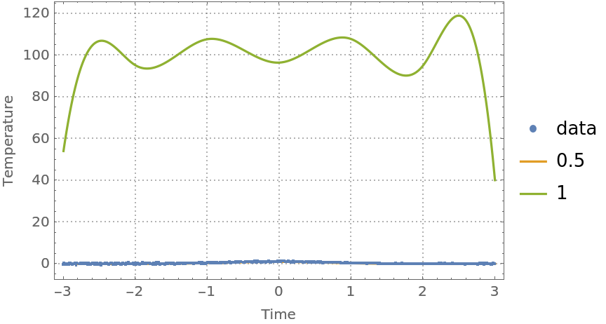 |
One way to fix this is to use probabilities that are close to 0 and 1 from above and below, respectively:
| In[43]:= | ![probs = {0.0001, 0.5, 0.9999};
qFuncs = ResourceFunction["QuantileRegression"][distData, 6, probs];
ListPlot[
Prepend[(Transpose[{distData[[All, 1]], #1 /@ distData[[All, 1]]}] &) /@ qFuncs, distData], Joined -> Prepend[Table[True, Length[probs]], False], PlotLegends -> Prepend[probs, "data"], PlotTheme -> "Detailed", FrameLabel -> {"Time", "Temperature"}, ImageSize -> Medium]](https://www.wolframcloud.com/obj/resourcesystem/images/5a6/5a6171c2-336f-4f2f-ad62-2baf3098c6b7/6a38b11fa0e3adb2.png) |
| Out[43]= | 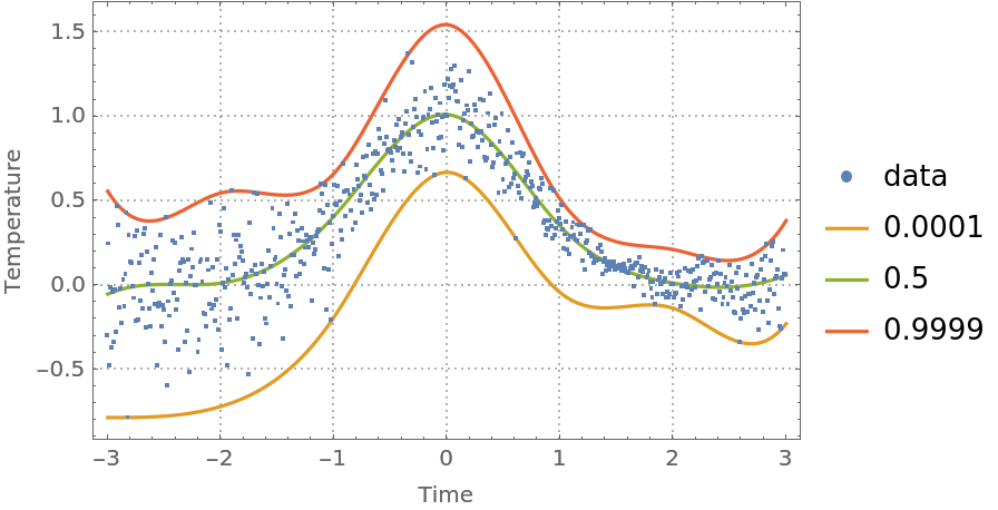 |
Consider the following nonlinear data:
| In[44]:= | ![nlData = {
Sequence[{0, 2.52}, {1., 2.83}, {2., 3}, {3., 3.2}, {4.1, 3.35}, {5., 3.47}, {6, 3.57}, {7, 3.66}, {8, 3.76}, {8.5, 3.81}, {9, 3.85}, {
9.5, 3.89}, {10.1, 3.94}, {10.5, 3.98}, {11, 4.01}, {11.5, 4.06}, {12, 4.09}, {12.5, 4.15}, {13, 4.19}, {13.5, 4.25}, {14, 4.3}, {14.5, 4.35}, {15, 4.41}, {15.6, 4.47}, {16, 4.53}, {16.5, 4.6}, {17., 4.68}, {17.5, 4.77}, {18, 4.85}, {18.5, 4.96}, {19, 5.11}, {19.55, 5.34}, {19.7,
5.44}, {19.9, 5.58}, {20.1, 5.91}, {20.3, 6.27}, {20.5, 7.14}, {
20.6, 7.14}, {20.8, 7.81}, {20.9, 8.32}, {21, 7.75}, {21.2, 9.07}, {21.4, 9.49}, {21.5, 9.71}, {21.6, 9.83}, {21.8, 10}, {22, 10.18}, {22.1, 10.21}, {22.2, 10.25}, {
22.3, 10.27}, {22.5, 10.3}, {22.7, 10.42}, {22.9, 10.47}, {23.1, 10.52}, {23.3, 10.59}, {23.5, 10.63}, {23.7, 10.67}, {24, 10.74}, {24.2, 10.78}, {24.4, 10.8}, {24.6, 10.82}, {
24.8, 10.84}, {25, 10.87}]};
ListPlot[nlData, Sequence[PlotTheme -> "Detailed", PlotStyle -> Red]]](https://www.wolframcloud.com/obj/resourcesystem/images/5a6/5a6171c2-336f-4f2f-ad62-2baf3098c6b7/21587cf3f2285905.png) |
| Out[44]= | 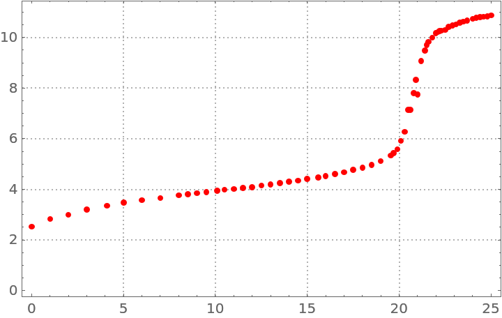 |
Make a quantile regression fit with 20 knots:
| In[45]:= |
Make a quantile regression fit with 40 knots:
| In[46]:= |
Plot the regression quantiles and the data:
| In[47]:= |
| Out[47]= | 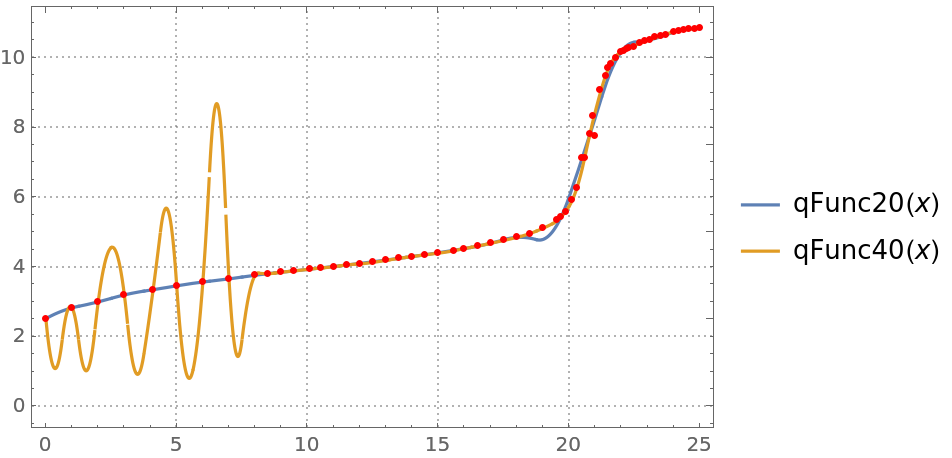 |
You can see that the regression quantile computed with 40 knots is "overfitted" between 0 and 8—the B-spline basis knots are too densely placed between 0 and 8.
When regression quantiles are overfitted, then the estimate of the conditional cumulative distribution function (CDF) can be problematic—the estimated CDF is not a monotonically increasing function.
Compute regression quantiles using "too many" knots:
| In[48]:= |
Plot the regression quantiles:
| In[49]:= | ![Block[{data = tempData[[1 ;; 300]]}, qFuncs = ResourceFunction["QuantileRegression"][data, 20, probs]; DateListPlot[
Prepend[(Transpose[{data[[All, 1]], #1 /@ data[[All, 1]]}] &) /@ qFuncs, data], Joined -> Prepend[Table[True, Length[probs]], False], PlotLegends -> Prepend[probs, "temperature data"], AspectRatio -> 1/4, PlotTheme -> "Detailed", FrameLabel -> {"Time", "Temperature"}, ImageSize -> Large]]](https://www.wolframcloud.com/obj/resourcesystem/images/5a6/5a6171c2-336f-4f2f-ad62-2baf3098c6b7/36a8a2ddb757d482.png) |
| Out[49]= | 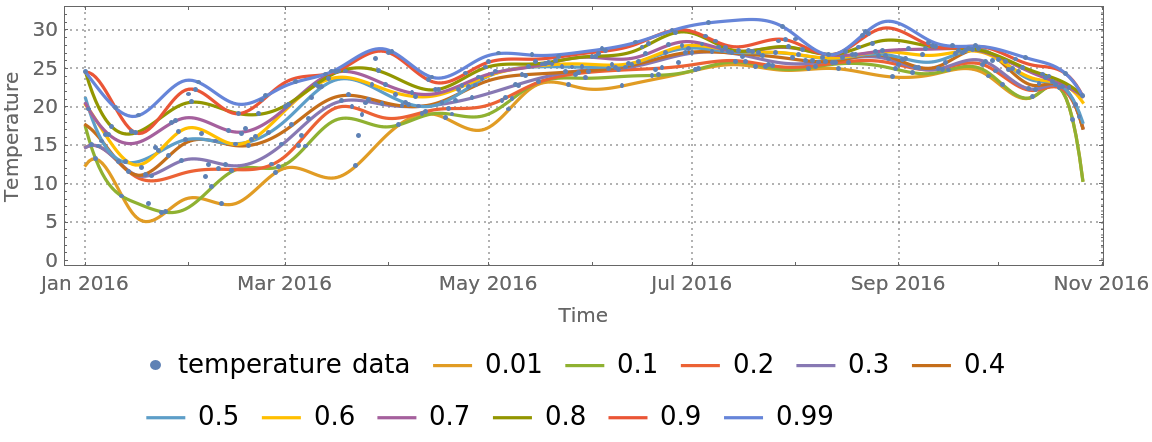 |
Here is the estimated conditional CDF:
| In[50]:= |
| Out[50]= | 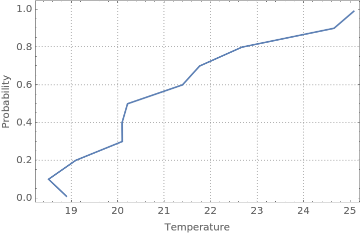 |
For certain data, it is beneficial to rescale the predictor values, predicted values, or both before doing the quantile regression computations:
| In[51]:= |  |
| In[52]:= |
| Out[52]= |
| In[53]:= |
| Out[53]= |
Compute and plot regression quantiles over symmetric data:
| In[54]:= | ![SeedRandom[20];
distData = Table[{x, Exp[-x^2] + RandomVariate[
NormalDistribution[0, .15 \[Sqrt](Abs[1.5 - x]/1.5)]]}, {x, -3, 3, .01}];
Grid[Table[Block[{tempData = RandomSample[distData, 100], data, probs},
data = Join[tempData, {#[[1]], -#[[2]]} & /@ tempData];
data = SortBy[Transpose[Rescale /@ Transpose[data]], #[[1]] &];
probs = {0.02, 0.48, 0.52, 0.98};
qFuncs = ResourceFunction["QuantileRegression"][data, 5, probs, Method -> {LinearProgramming, Method -> "InteriorPoint", Tolerance -> 10^(-2)}]; ListPlot[
Prepend[(Transpose[{data[[All, 1]], #1 /@ data[[All, 1]]}] &) /@ qFuncs, data], Joined -> Prepend[Table[True, Length[probs]], False], Filling -> Prepend[Table[(i + 1) -> {i + 2}, {i, Length[probs] - 1}], 1 -> None], Frame -> True, FrameTicks -> False, Axes -> False, ImageSize -> Small, AspectRatio -> 1]
], 3, 3]]](https://www.wolframcloud.com/obj/resourcesystem/images/5a6/5a6171c2-336f-4f2f-ad62-2baf3098c6b7/599d3e658927fc99.png) |
| Out[54]= | 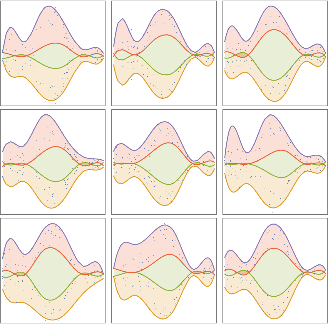 |
This work is licensed under a Creative Commons Attribution 4.0 International License