Basic Examples (8) 

A system that starts at -1:

In[1]:=

The state and input weights:

In[2]:=

The initial value of the gain:

In[3]:=

The total simulations is 30 with a batch consisting of 10 simulations:

In[4]:=

Compute the controller:

In[5]:=

Out[5]=

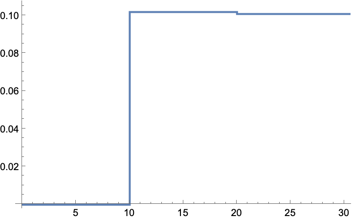
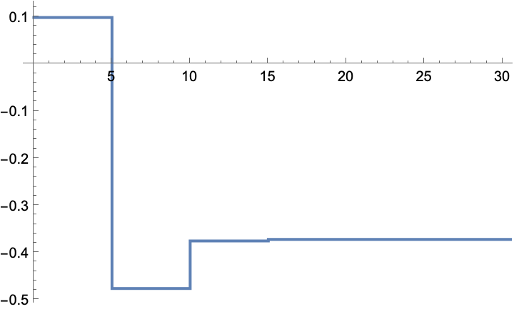
The gain converges to ~0.1:

In[6]:=

Out[6]=

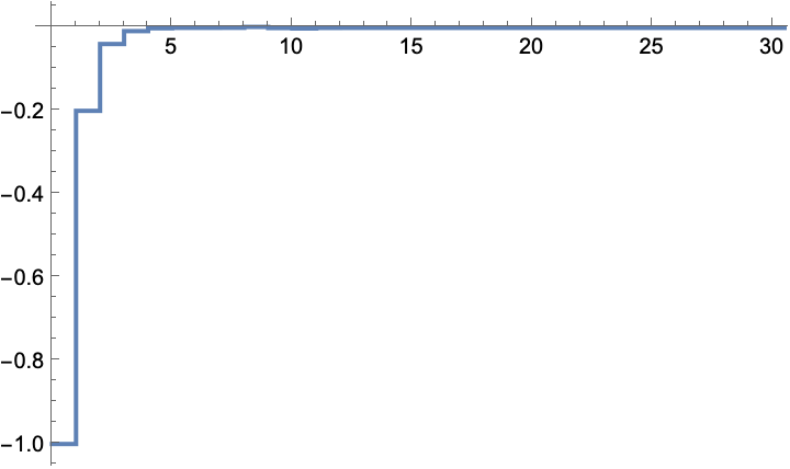
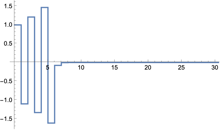
The state is regulated to the origin:

In[7]:=

Out[7]=

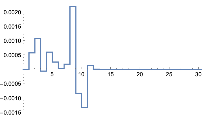
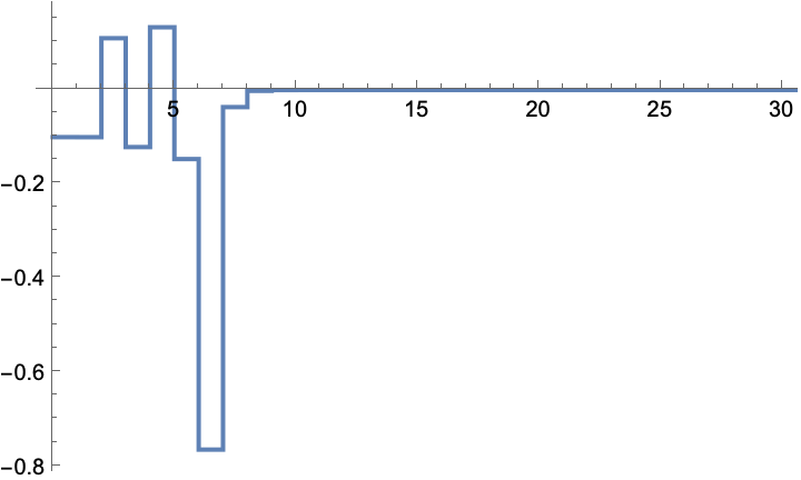
The input sequence that was used during the simulation:

In[8]:=

Out[8]=

Scope (6) 

A system with one state and one input:

In[9]:=

Compute a controller:

In[10]:=

Out[10]=

The gain values:

In[11]:=

Out[11]=

The state is regulated to the origin:

In[12]:=

Out[12]=

The input sequence that was used during the simulation:

In[13]:=

Out[13]=

A multi-state system:

In[14]:=

Compute a controller:

In[15]:=

Out[15]=

The gain values:

In[16]:=

Out[16]=

The states are regulated to the origin:

In[17]:=

Out[17]=

The input sequence that was used during the simulation:

In[18]:=

Out[18]=

A multi-state, multi-input system:

In[19]:=

Compute a controller:

In[20]:=

Out[20]=

The gain values:

In[21]:=

Out[21]=

The states are regulated to the origin:

In[22]:=

Out[22]=

The input sequence that was used during the simulation:

In[23]:=

Out[23]=

A state-space model:

In[24]:=

Compute a controller:

In[25]:=

Out[25]=

The gain values:

In[26]:=

Out[26]=

The states are regulated to the origin:

In[27]:=

Out[27]=

The input sequence that was used during the simulation:

In[28]:=

Out[28]=

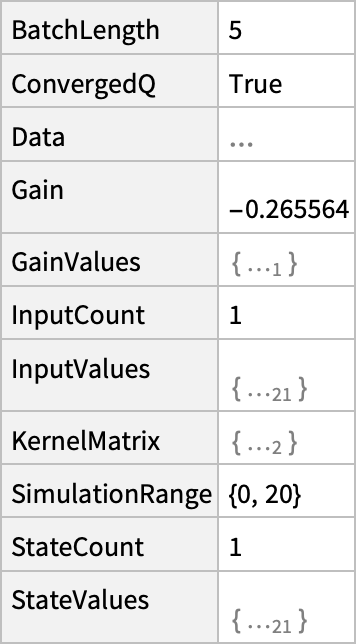
By default, a SystemsModelControllerData object is returned:

In[29]:=

Out[29]=

It can be used to obtain various properties:

In[30]:=

Out[30]=

The value of a specific property:

In[31]:=

Out[31]=

A list of property values:

In[32]:=

Out[32]=

The values of all properties as an Association:

In[33]:=

Out[33]=

As a Dataset:

In[34]:=

Out[34]=

Get a property directly:

In[35]:=

Out[35]=

Applications (7) 

The model of the U.S Coast Guard cutter Tampa based on sea-trials data that gives the heading in response to rudder angle inputs:

In[36]:=

Out[36]=

Discretize the model:

In[37]:=

Out[37]=

The model is marginally stable:

In[38]:=

Out[38]=

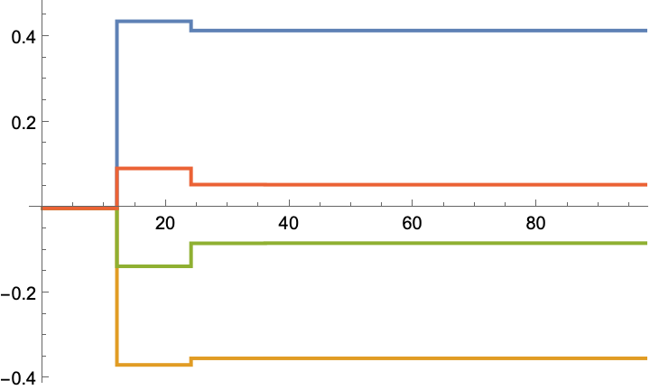
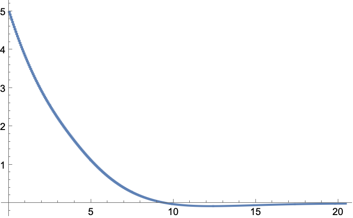
A Q-learning LQ regulator starting with an initial heading of 5°:

In[39]:=

Out[39]=

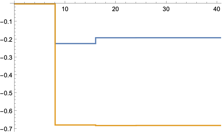
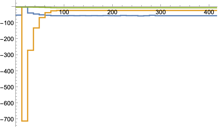
The computed gain values:

In[40]:=

Out[40]=

The heading is regulated back to the origin in about 20 seconds:

In[41]:=

Out[41]=

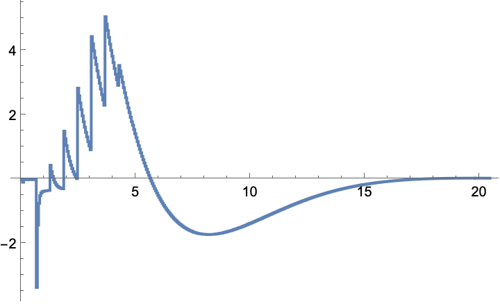
The rudder input values:

In[42]:=

Out[42]=

Properties and Relations (2) 

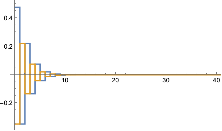
The gain computed by simulation converges to the optimal solution:

In[43]:=

In[44]:=

In[45]:=

Out[45]=

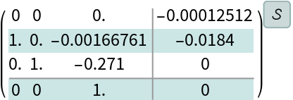
The optimal solution computed with knowledge of the system's dynamics:

In[46]:=

Out[46]=

The above solution is computed using the discrete algebraic Riccati equation:

In[47]:=

Out[47]=

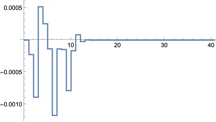
The gain computed by simulation converges to the optimal solution for a nonlinear system:

In[48]:=

In[49]:=

In[50]:=

Out[50]=

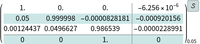
The optimal solution computed using the linearized model:

In[51]:=

Out[51]=

The above solution is computed using the discrete algebraic Riccati equation:

In[52]:=

In[53]:=

Out[53]=

Possible Issues (4) 

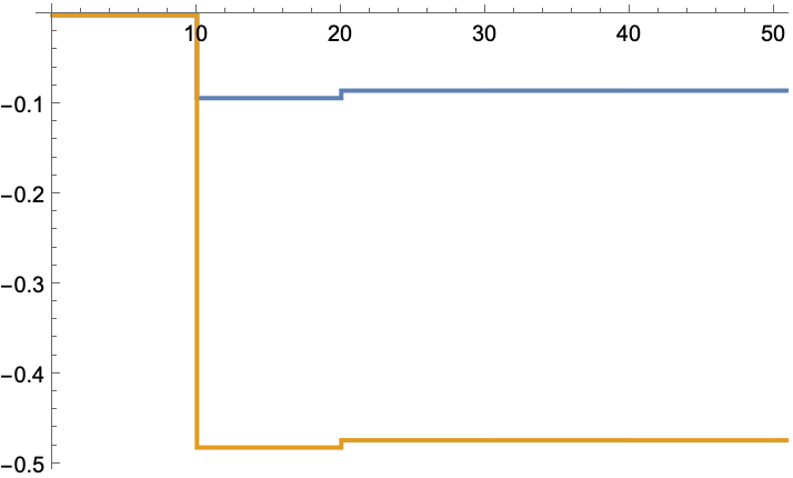
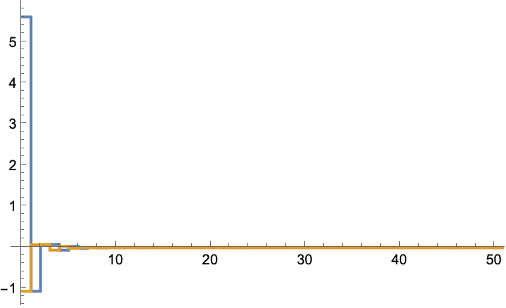
An unstable system may not converge to the optimal solution:

In[54]:=

In[55]:=

Out[55]=

Adjusting the initial gain causes it to converge to the optimal solution:

In[56]:=

Out[56]=

The optimal solution:

In[57]:=

Out[57]=

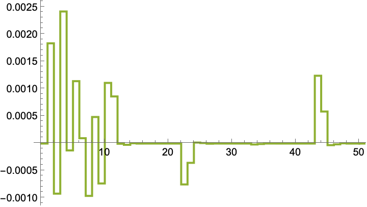
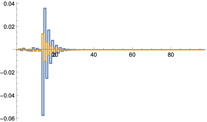
A system with a disturbance may not converge to the optimal solution:

In[58]:=

In[59]:=

Out[59]=

Adjusting the initial gain may cause it to come close to the optimal solution:

In[60]:=

Out[60]=

The optimal solution:

In[61]:=

Out[61]=

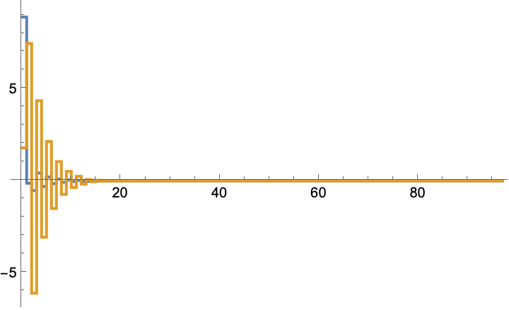
The initial gain must be stabilizing:

In[62]:=

Otherwise the state values will blow up:

In[63]:=

Out[63]=

The state values with a stabilizing gain:

In[64]:=

Out[64]=

The system must be a discrete-time system:

In[65]:=

Out[65]=

In[66]:=

Out[66]=