Wolfram Function Repository
Instant-use add-on functions for the Wolfram Language
Function Repository Resource:
Plot a predator-prey pursuit curve
ResourceFunction["PursuitCurvePlot"][c,p,{t,t0,tf}] plots the pursuit curve of a predator starting at a point p, moving in the direction of the current position of the prey, following a path c from time t0 to time tf. |
| "DirectionOfMotion" | plot vectors in the directions of motion of the predator and the prey |
| "PredatorPreyVectorSet" | plot a set of vectors from the predator to the prey as the curve evolves |
Plot the pursuit curve for linear motion with unit speed:
| In[1]:= |
| Out[1]= | 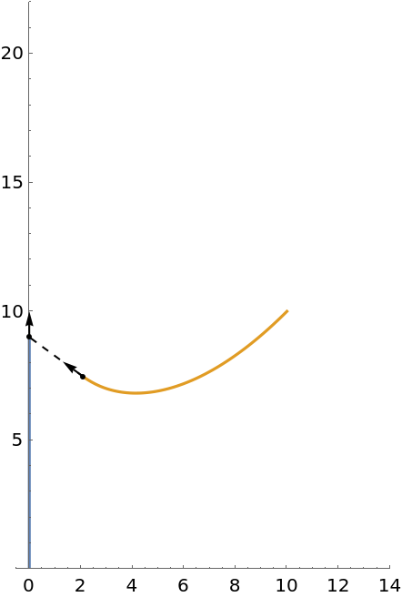 |
Animate the pursuit curve over time:
| In[2]:= | ![Animate[ResourceFunction[
"PursuitCurvePlot"][{0, t}, {10, 10}, {t, 0., n}, PlotRange -> {{-.5, 14}, {0, 22}}], {{n, 1}, 1, 21, .1}]](https://www.wolframcloud.com/obj/resourcesystem/images/94b/94b049a6-7e57-418a-aba3-12d9dda10183/1428af955dca83e2.png) |
| Out[2]= | 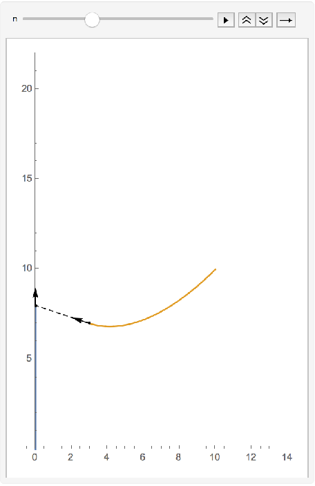 |
Plot the pursuit curve for circular motion:
| In[3]:= |
| Out[3]= | 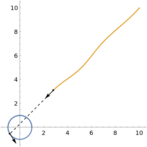 |
Manipulate the curve evolution via the time parameter:
| In[4]:= | ![Manipulate[
ResourceFunction[
"PursuitCurvePlot"][{Cos[t], Sin[t]}, {10, 10}, {0, 1}, {t, 0., tf},
PlotRange -> {{-2., 10.`}, {-2., 10.`}}], {{tf, 12}, 0.1, 15}]](https://www.wolframcloud.com/obj/resourcesystem/images/94b/94b049a6-7e57-418a-aba3-12d9dda10183/2bc1d4e66d826c29.png) |
| Out[4]= | 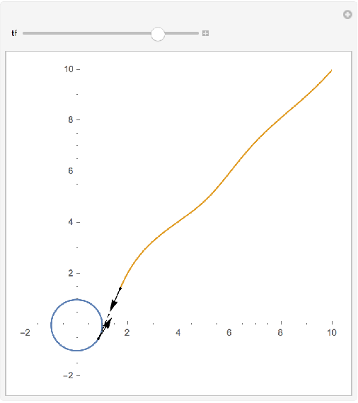 |
A case where the predator never reaches the prey:
| In[5]:= | ![ResourceFunction[
"PursuitCurvePlot"][{Cos[t], Sin[t]}, {-7., 1.}, {t, 0., 500.}, "PursuitCurveDataFunction" -> ({PointSize[0.03`], MapThread[{#2, Point[#1]} &, {#3, {Red, Blue}}]} &)]](https://www.wolframcloud.com/obj/resourcesystem/images/94b/94b049a6-7e57-418a-aba3-12d9dda10183/64043f30be4211b7.png) |
| Out[5]= | 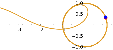 |
Use a figure-eight prey curve:
| In[6]:= | ![Manipulate[
ResourceFunction["PursuitCurvePlot"][{Cos[5 t], Cos[5 t] Sin[5 t]}, xy0, {t, 0., tf}, PlotRange -> 3], {{xy0, {-0.8, 0.2}, "initial position predator"}, {-3, -3}, {3, 3}}, {{tf, 29.5}, .1, 60}, ControlPlacement -> Top]](https://www.wolframcloud.com/obj/resourcesystem/images/94b/94b049a6-7e57-418a-aba3-12d9dda10183/0e09c33731265b9c.png) |
| Out[6]= | 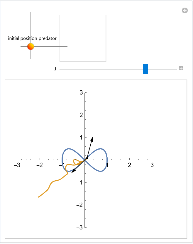 |
Use a gradient of colors for the curve:
| In[7]:= |
| Out[7]= | 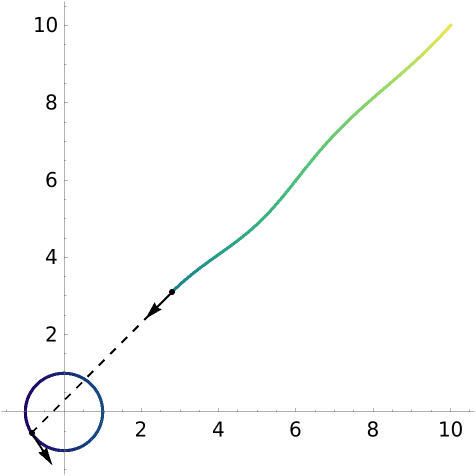 |
Remove the vectors:
| In[8]:= |
| Out[8]= | 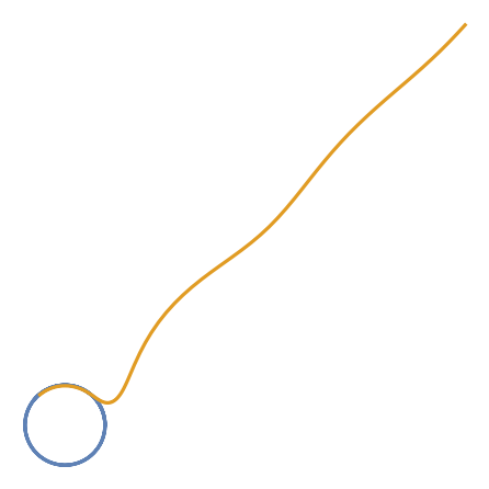 |
Use a custom function to put points for current positions:
| In[9]:= | ![ResourceFunction[
"PursuitCurvePlot"][{Cos[t], Sin[t]}, {10, 10}, {t, 0., 12.}, "PursuitCurveDataFunction" -> ({PointSize[.03], MapThread[{#2, Point[#1]} &, {#3, {Red, Blue}}]} &)]](https://www.wolframcloud.com/obj/resourcesystem/images/94b/94b049a6-7e57-418a-aba3-12d9dda10183/7e9f6eeddf5e02d6.png) |
| Out[9]= | 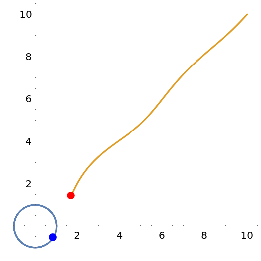 |
Include a plot of the distance between predator and prey:
| In[10]:= | ![Module[{\[Alpha] = 0.014}, ResourceFunction[
"PursuitCurvePlot"][{Cos[t], Cos[t] Sin[t]}, {2.2, -2.7}, {\[Alpha],
0.646}, {t, 0., 23.}, Axes -> False, PlotRange -> {{-1., 1.}, {-1.4, .6}}, "PursuitCurveDataFunction" -> (Inset[(plot = Plot[Evaluate[
Norm[{(1 - \[Alpha] t) Cos[t] - x[t], (1 - \[Alpha] t) Cos[t] Sin[t] - y[t]}] /. #1[[
1]]], {t, 0, #2}, PlotLabel -> Row[{"t", #2}, "="], PlotRange -> {Automatic, {0, 1.1}}, AxesOrigin -> {0, 0}]), {-.8, -1.1}, {.3, .3}] &)]]](https://www.wolframcloud.com/obj/resourcesystem/images/94b/94b049a6-7e57-418a-aba3-12d9dda10183/5c6a57362f900f6c.png) |
| Out[10]= | 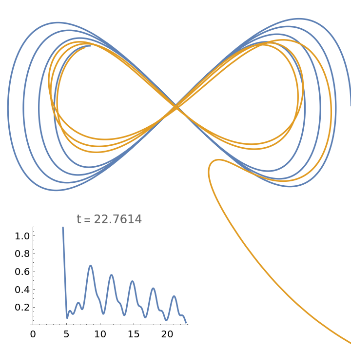 |
Plot a set of vectors between the predator and the prey along the evolution of the curves:
| In[11]:= | ![Module[{tf = 24, xy0 = {2.2, -2.7}, \[Alpha] = 0.014, \[Beta] = 0.646}, ResourceFunction[
"PursuitCurvePlot"][{Cos[t], Cos[t] Sin[t]}, {1.8, -2.}, {\[Alpha], \[Beta]}, {t, 0, tf}, "PursuitCurveDataFunction" -> "PredatorPreyVectors", Axes -> False, PlotRange -> All]]](https://www.wolframcloud.com/obj/resourcesystem/images/94b/94b049a6-7e57-418a-aba3-12d9dda10183/3fc642927ca720cd.png) |
| Out[11]= | 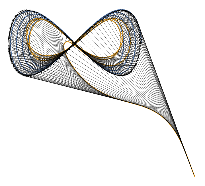 |
This work is licensed under a Creative Commons Attribution 4.0 International License