Wolfram Function Repository
Instant-use add-on functions for the Wolfram Language
Function Repository Resource:
Evaluate the radial pseudo-Zernike polynomial
ResourceFunction["PseudoZernikeR"][n,m,r] gives the radial pseudo-Zernike polynomial |
Evaluate numerically:
| In[1]:= |
| Out[1]= |
Evaluate symbolically:
| In[2]:= |
| Out[2]= |
Plot over a subset of the reals:
| In[3]:= |
| Out[3]= | 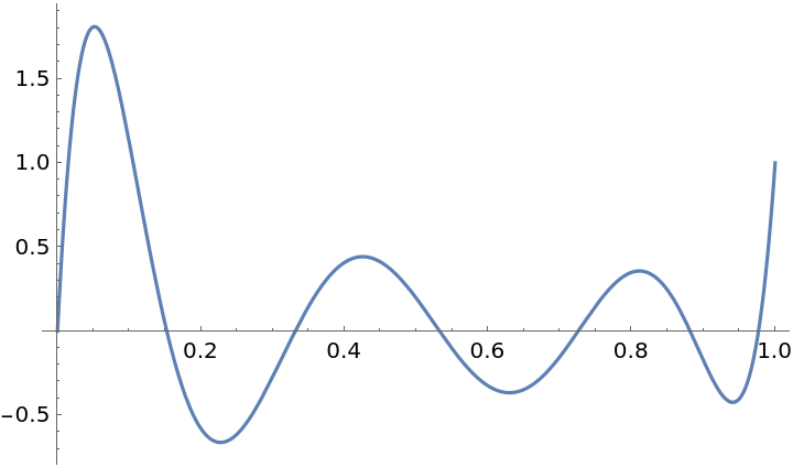 |
Evaluate to high precision:
| In[4]:= |
| Out[4]= |
The precision of the output tracks the precision of the input:
| In[5]:= |
| Out[5]= |
Simple exact values are generated automatically:
| In[6]:= |
| Out[6]= |
PseudoZernikeR threads elementwise over lists:
| In[7]:= |
| Out[7]= |
Obtain the pseudo-Zernike polynomials from their generating function:
| In[8]:= | ![m = 3; Series[(
2^(2 m + 1) r^m)/((1 + t + Sqrt[1 + 2 (1 - 2 r) t + t^2])^(2 m + 1)
Sqrt[1 + 2 (1 - 2 r) t + t^2]), {t, 0, 5}]](https://www.wolframcloud.com/obj/resourcesystem/images/c84/c8425a34-d3ba-42df-8bef-72c1a1be8aaa/37b7c6ecc1cf8c48.png) |
| Out[8]= |
| In[9]:= |
| Out[9]= |
Compare with the directly computed sequence:
| In[10]:= |
| Out[10]= |
Verify an expression for the pseudo-Zernike polynomial in terms of the Jacobi polynomial JacobiP:
| In[11]:= | ![Table[ResourceFunction["PseudoZernikeR"][n, m, r] == r^m (-1)^(n - m) JacobiP[n - m, 2 m + 1, 0, 1 - 2 r] // Simplify, {n, 0, 5}, {m, 0, n}]](https://www.wolframcloud.com/obj/resourcesystem/images/c84/c8425a34-d3ba-42df-8bef-72c1a1be8aaa/289a59660b4b57bc.png) |
| Out[11]= |
Verify a recurrence relation for the pseudo-Zernike polynomials:
| In[12]:= | ![Table[ResourceFunction["PseudoZernikeR"][n + 1, m, r] == (
2 n + 3)/((n + m + 2) (n - m + 1)) ((2 (n + 1) r - (n + m + 1)^2/(2 n + 1) - (n - m + 1)^2/(
2 n + 3)) ResourceFunction["PseudoZernikeR"][n, m, r] - ((n + m + 1) (n - m))/(2 n + 1)
ResourceFunction["PseudoZernikeR"][n - 1, m, r]) // Simplify, {n, 5}, {m, 0, n - 1}]](https://www.wolframcloud.com/obj/resourcesystem/images/c84/c8425a34-d3ba-42df-8bef-72c1a1be8aaa/2e6ab85cfe9f720a.png) |
| Out[12]= |
Verify the orthogonality relation for the pseudo-Zernike polynomials:
| In[13]:= | ![MatrixForm /@ Table[2 (n1 + 1) Integrate[
r ResourceFunction["PseudoZernikeR"][n1, m, r] ResourceFunction[
"PseudoZernikeR"][n2, m, r], {r, 0, 1}], {m, 0, 3}, {n1, m, m + 3}, {n2, m, m + 3}]](https://www.wolframcloud.com/obj/resourcesystem/images/c84/c8425a34-d3ba-42df-8bef-72c1a1be8aaa/24c0cca6eb4487ce.png) |
| Out[13]= |  |
Visualize pseudo-Zernike polynomials over the unit disk:
| In[14]:= | ![Table[DensityPlot[
ResourceFunction["PseudoZernikeR"][n, m, Norm[{x, y}]] Cos[
m ArcTan[x, y]], {x, y} \[Element] Disk[], ColorFunction -> (ColorData[{"ThermometerColors", "Reverse"}, LogisticSigmoid[2 #]] &), ColorFunctionScaling -> False, Exclusions -> None, Frame -> False, PlotPoints -> 55], {n, 0, 4}, {m, 0, n}] // GraphicsGrid](https://www.wolframcloud.com/obj/resourcesystem/images/c84/c8425a34-d3ba-42df-8bef-72c1a1be8aaa/6cd9d59f8abf4dd5.png) |
| Out[14]= | 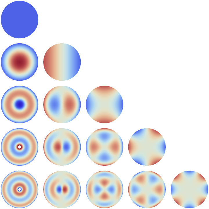 |
This work is licensed under a Creative Commons Attribution 4.0 International License