Wolfram Function Repository
Instant-use add-on functions for the Wolfram Language
Function Repository Resource:
PythonObject configuration for the Python package ProbNum
ResourceFunction["ProbNumObject"][] returns a configured PythonObject for the Python package ProbNum in a new Python session. | |
ResourceFunction["ProbNumObject"][session] uses the specified running ExternalSessionObject session. | |
ResourceFunction["ProbNumObject"][…,"func"[args,opts]] executes the function func with the specified arguments and options. |
| Linear solvers | solve Ax=b for x |
| ODE solvers | solve f(y(t),t) for y |
| Integral solvers | solve |
| p | the same Python object p for all ti |
| {p1,p2,…} | respective pi for ti |
| plist | a Python object representing a Python-side list of models |
| "RNG" | access the random number generator |
| “MeanPlots" | plot mean solution values |
| "SamplePlots" | plot ODE solution samples |
| "UncertaintyBandPlots" | plot uncertainty bands |
Solve a linear matrix equation:
| In[1]:= |
| In[2]:= |
| Out[2]= |  |
| In[3]:= |
| Out[3]= |  |
The multivariate Gaussian random variable corresponding to the solution:
| In[4]:= |
| Out[4]= |  |
The mean of the normal distribution equals the best guess for the solution of the linear system:
| In[5]:= |
| Out[5]= |
The covariance matrix provides a measure of uncertainty:
| In[6]:= |
| Out[6]= |
In this case, the algorithm is very certain about the solution as the covariance matrix is virtually zero:
| In[7]:= |
| Out[7]= |
Clean up by closing the Python session:
| In[8]:= |
Deploy a Python function describing an ODE vector field in a Python session:
| In[9]:= |
| Out[9]= |
| In[10]:= |
| Out[10]= |
Create a ProbNum Python object:
| In[11]:= |
| Out[11]= |  |
Solve the logistic ODE corresponding the field f with time running from t0 to tmax given the initial value vector y0:
| In[12]:= |
| In[13]:= |
| Out[13]= |  |
Obtain numerical values:
| In[14]:= |
| Out[14]= |
Plot the solution:
| In[15]:= |
| Out[15]= | 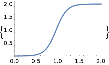 |
The uncertainty band around the solution is quite narrow indicating a high degree of certainty:
| In[16]:= |
| Out[16]= | 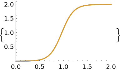 |
| In[17]:= |
Deploy a function in a Python session:
| In[18]:= |
| Out[18]= |
| In[19]:= |
| Out[19]= |
| In[20]:= |
| Out[20]= |
Create a ProbNum Python object:
| In[21]:= |
| Out[21]= |  |
| In[22]:= |
| In[23]:= |
| Out[23]= |  |
| In[24]:= |
| Out[24]= |  |
The mean value and standard deviation of the random variable represent the result of integration:
| In[25]:= |
| Out[25]= |
| In[26]:= |
| Out[26]= |
Additional information in bqinfo:
| In[27]:= |
| Out[27]= |
| In[28]:= |
| Out[28]= |
Compare with NIntegrate:
| In[29]:= |
| Out[29]= |
Clean up:
| In[30]:= |
Generate a random symmetric positive definite matrix with a given spectrum, seeding the random number generator for reproducibility:
| In[31]:= |
| Out[31]= |  |
| In[32]:= |
| Out[32]= |  |
| In[33]:= |
| In[34]:= |
| Out[34]= |
| In[35]:= |
| Out[35]= |  |
Define a random n⨯1 matrix:
| In[36]:= |
Visualize the linear system formed by the matrices:
| In[37]:= |
| Out[37]= | 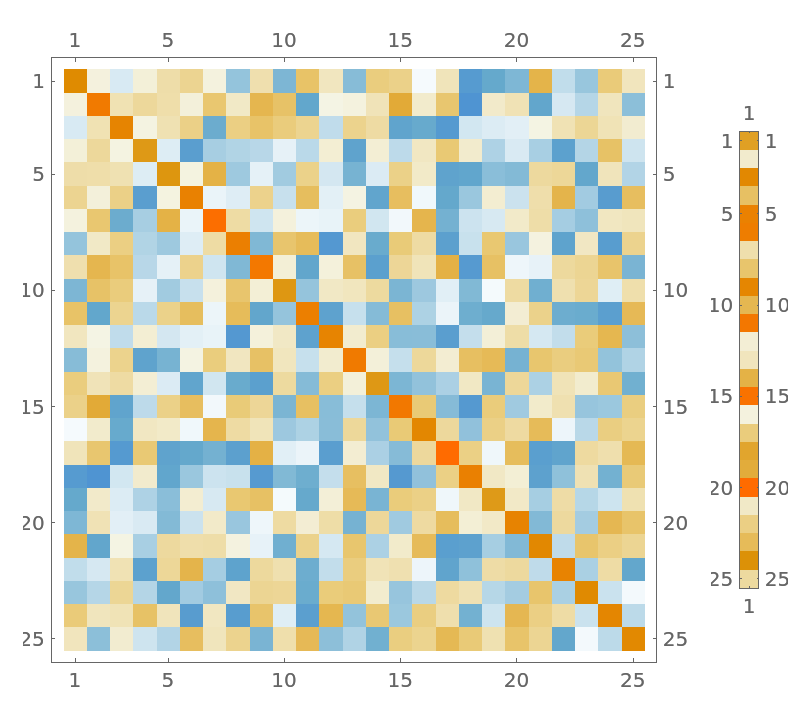 |
Solve the linear system a.x==b in a Bayesian framework using 10 iterations:
| In[38]:= |
| Out[38]= | 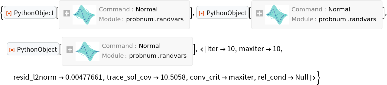 |
The mean of the random variable x is the “best guess” for the solution:
| In[39]:= |
| Out[39]= |
Plot mean values of elements of the solution along with 68% credible intervals which capture per element distributions of x:
| In[40]:= |
| Out[40]= | 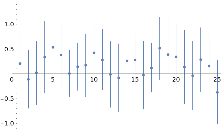 |
Samples from the normal distribution give possible solution vectors x1, x2, … which take into account cross correlations between the entries:
| In[41]:= |
| Out[41]= | 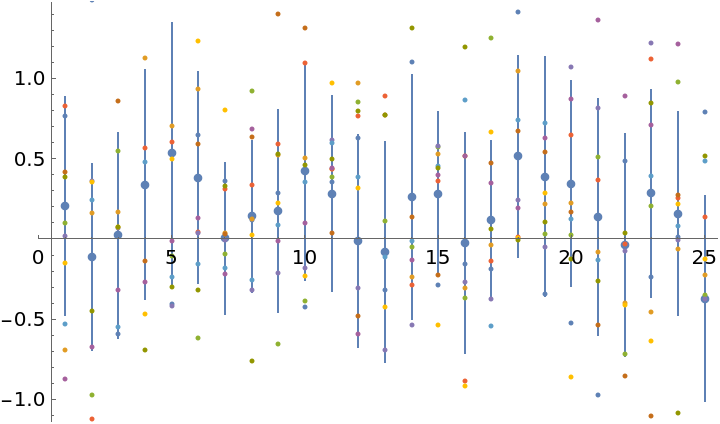 |
A more accurate solution can be obtained with more iterations or, for this system, with LinearSolve:
| In[42]:= |
Even after 10 iterations, the ProbNum "best guess" solution is very close to the "true" solution:
| In[43]:= |
| Out[43]= | 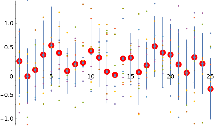 |
Maximal absolute and relative errors of the mean estimate:
| In[44]:= |
| Out[44]= |
The inverse of the matrix a looks close to its estimate ai. The latter maybe useful when obtaining the inverse directly is infeasible:
| In[45]:= |
| Out[45]= | 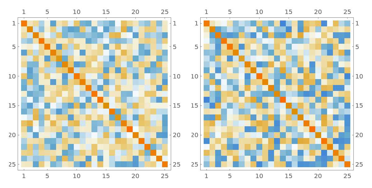 |
| In[46]:= |
Open a Python session:
| In[47]:= |
| Out[47]= |
| In[48]:= |
| Out[48]= |  |
Define a vector field:
| In[49]:= |
| Out[49]= |
Solve an initial value problem (IVP) with a filtering-based probabilistic ODE solver using fixed steps:
| In[50]:= |
| In[51]:= |
| Out[51]= |  |
The mean of the discrete-time solution:
| In[52]:= |
| Out[52]= |
The time grid:
| In[53]:= |
| Out[53]= |
Plot the solution:
| In[54]:= |
| Out[54]= | 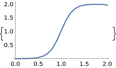 |
Construct and plot an interpolation corresponding to the continuous-time solution:
| In[55]:= | ![Interpolation[
Transpose[{solution["locations"] // Normal // Normal, solution["states"]["mean"] // Normal // Normal}]]](https://www.wolframcloud.com/obj/resourcesystem/images/00e/00e34b5b-0d17-4b80-8821-92f7741a4e49/21e2937abf4aa856.png) |
| Out[55]= |
| In[56]:= |
| Out[56]= | 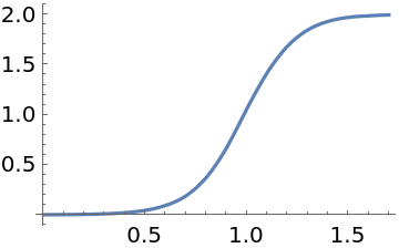 |
| In[57]:= |
Solve the same problem using the first-order extended Kalman filtering/smoothing:
| In[58]:= |
| In[59]:= |
Vector field:
| In[60]:= |
| Out[60]= |
The Jacobian of the ODE vector field:
| In[61]:= |
| Out[61]= |
Solve the initial value problem:
| In[62]:= |
| In[63]:= | ![solution = p["ProbabilisticSolveIVP"[f, t0, tmax, y0, "Df" -> df, Method -> "EK1", "AlgorithmOrder" -> 2, "Step" -> 0.1, "Adaptive" -> False]]](https://www.wolframcloud.com/obj/resourcesystem/images/00e/00e34b5b-0d17-4b80-8821-92f7741a4e49/51f86d68dd6f994d.png) |
| Out[63]= |  |
Plot the solution:
| In[64]:= |
| Out[64]= | 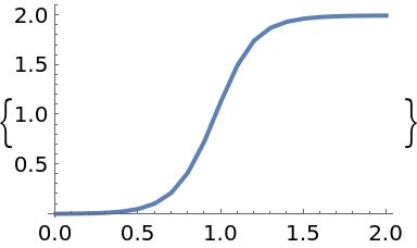 |
Clean up:
| In[65]:= |
Define the ODE for the Lotka-Volterra prey-predators problem:
| In[66]:= |
| In[67]:= |
| In[68]:= | ![f = ResourceFunction["ToPythonFunction"][session, Function[{t, y}, {0.5` y[[1]] - 0.05` y[[1]] y[[2]], -0.5` y[[2]] + 0.05` y[[1]] y[[2]]}], Method -> "np"]](https://www.wolframcloud.com/obj/resourcesystem/images/00e/00e34b5b-0d17-4b80-8821-92f7741a4e49/48f976aadd060f30.png) |
| Out[68]= | 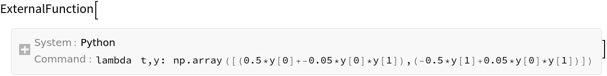 |
| In[69]:= | ![df = ResourceFunction["ToPythonFunction"][session, Function[{t, y}, {{0.5` - 0.05` y[[2]], -0.05` y[[1]]}, {0.05` y[[2]], -0.5` + 0.05` y[[1]]}}], Method -> "np"]](https://www.wolframcloud.com/obj/resourcesystem/images/00e/00e34b5b-0d17-4b80-8821-92f7741a4e49/62b9f585f895f0a1.png) |
| Out[69]= | 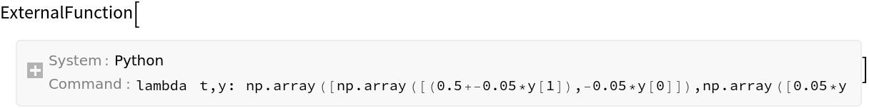 |
Solve with adaptive steps:
| In[70]:= |
| In[71]:= |
| Out[71]= |  |
Combine plots and notice smaller steps near solution peaks:
| In[72]:= | ![plot[solution_] := Show[MapThread[
Legended[Show[# /. _RGBColor -> #2, Frame -> True], LineLegend[{#2}, {#3}]] &, {ResourceFunction["ProbNumObject"][
"MeanPlots"[solution, PlotLabel -> None]], {Darker[Green], Orange}, {"Prey", "Predators"}}], GridLines -> {solution["locations"] // Normal // Normal, Automatic}]](https://www.wolframcloud.com/obj/resourcesystem/images/00e/00e34b5b-0d17-4b80-8821-92f7741a4e49/355172effd37b85b.png) |
| In[73]:= |
| Out[73]= | 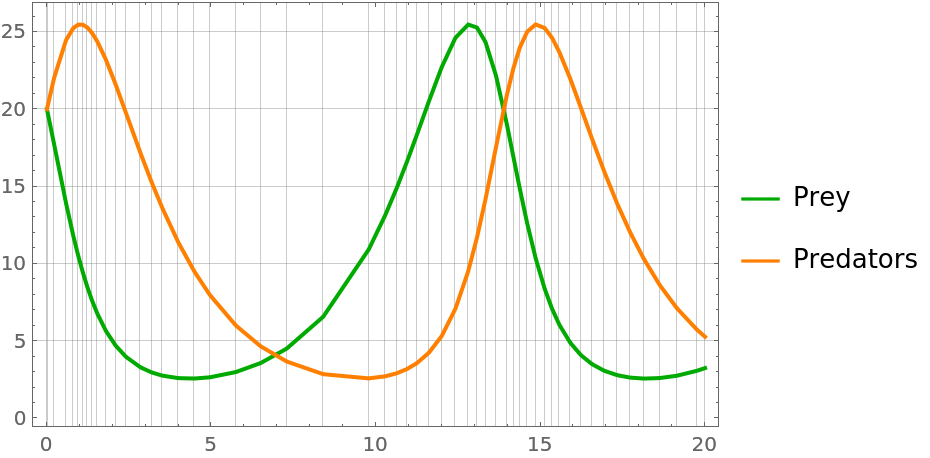 |
The higher-order filters takes fewer steps than the lower-order ones:
| In[74]:= | ![GraphicsGrid@
Table[Show[
plot[p["ProbabilisticSolveIVP"[f, t0, tmax, y0, "Df" -> df, Method -> filter, "AlgorithmOrder" -> order]]] //. Legended[pl_, _] :> pl, PlotLabel -> StringTemplate["Order `order` with `filter`"][<|"order" -> order, "filter" -> filter|>]], {order, {2, 3}}, {filter, {"EK0", "EK1"}}]](https://www.wolframcloud.com/obj/resourcesystem/images/00e/00e34b5b-0d17-4b80-8821-92f7741a4e49/15fcaec295a2b1d8.png) |
| Out[74]= | 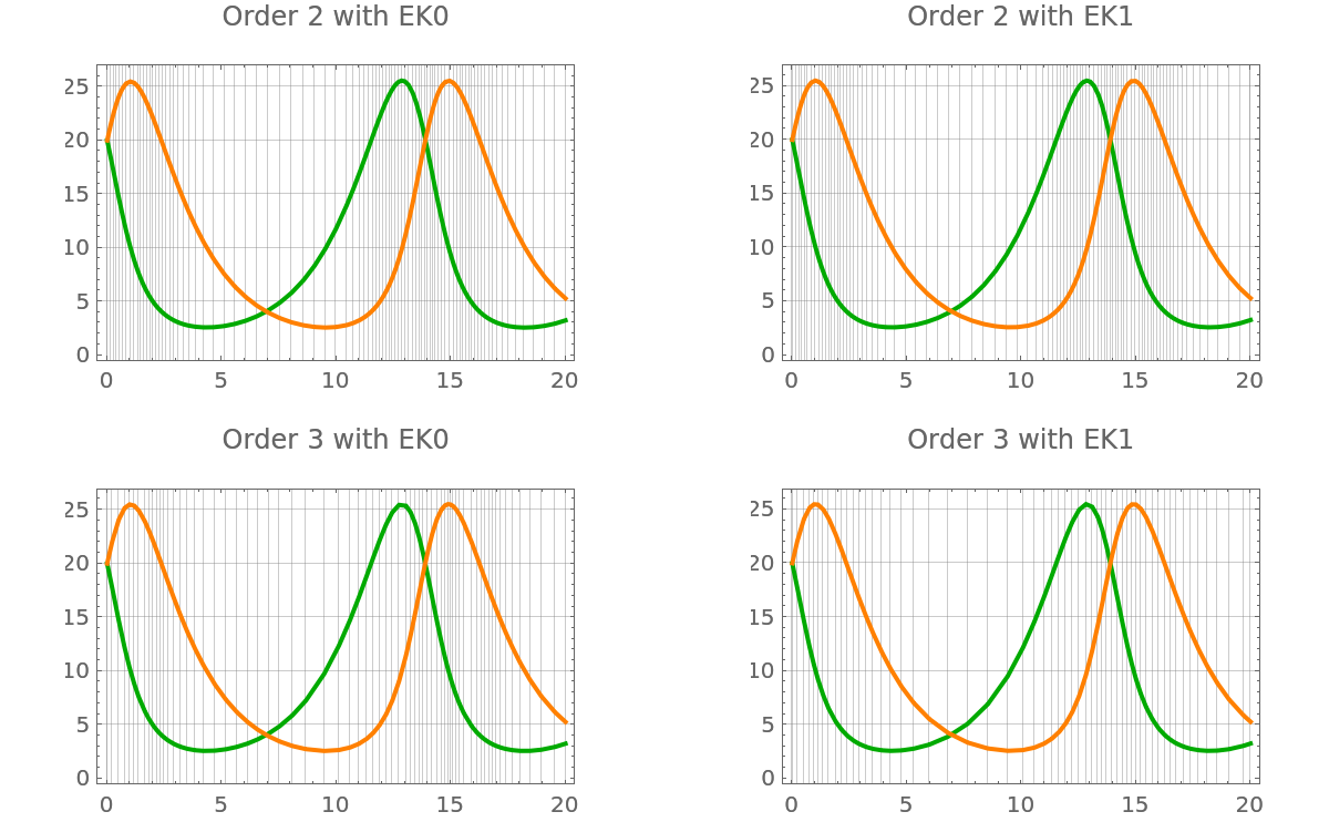 |
| In[75]:= |
To investigate uncertainties of the ODE solution, consider the same prey-predators problem:
| In[76]:= |
| In[77]:= |
| In[78]:= | ![f = ResourceFunction["ToPythonFunction"][session, Function[{t, y}, {0.5` y[[1]] - 0.05` y[[1]] y[[2]], -0.5` y[[2]] + 0.05` y[[1]] y[[2]]}], Method -> "np"];](https://www.wolframcloud.com/obj/resourcesystem/images/00e/00e34b5b-0d17-4b80-8821-92f7741a4e49/1420161a259dc5e3.png) |
| In[79]:= | ![df = ResourceFunction["ToPythonFunction"][session, Function[{t, y}, {{0.5` - 0.05` y[[2]], -0.05` y[[1]]}, {0.05` y[[2]], -0.5` + 0.05` y[[1]]}}], Method -> "np"];](https://www.wolframcloud.com/obj/resourcesystem/images/00e/00e34b5b-0d17-4b80-8821-92f7741a4e49/685bab4d4e411713.png) |
Obtain a low-resolution solution so that uncertainties are better visible:
| In[80]:= |
| In[81]:= | ![solution = p["ProbabilisticSolveIVP"[f, t0, tmax, y0, "Df" -> df, "AlgorithmOrder" -> 1, "Step" -> .5, "Adaptive" -> False, "diffusion_model" -> "dynamic"]]](https://www.wolframcloud.com/obj/resourcesystem/images/00e/00e34b5b-0d17-4b80-8821-92f7741a4e49/4c17fb50d4ea766c.png) |
| Out[81]= |  |
Prepare plots of uncertainty bands and a few samples from the solution:
| In[82]:= |
| Out[82]= |  |
| In[83]:= |
| In[84]:= |
Display the plots and notice that uncertainties are higher in valleys than in peaks; they also increase over time:
| In[85]:= |
| Out[85]= | 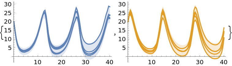 |
| In[86]:= |
Solve an initial value problem with a perturbation-based probabilistic ODE solver:
| In[87]:= |
| In[88]:= |
| Out[88]= |
| In[89]:= |
| Out[89]= |  |
| In[90]:= |
| In[91]:= |
| Out[91]= |  |
| In[92]:= | ![solution = p["PerturbationSolveIVP"[f, t0, tmax, y0, rng, "Step" -> 0.25, Method -> "RK23", "Adaptive" -> False]]](https://www.wolframcloud.com/obj/resourcesystem/images/00e/00e34b5b-0d17-4b80-8821-92f7741a4e49/13ceaa58dd5d4210.png) |
| Out[92]= |  |
Plot the solution:
| In[93]:= |
| Out[93]= |  |
Each solution is the result of a randomly-perturbed call of an underlying Runge-Kutta solver. Therefore, the output is different for successive calls:
| In[94]:= | ![Show[Table[
ResourceFunction["ProbNumObject"][
"MeanPlots"[
p["PerturbationSolveIVP"[f, t0, tmax, y0, rng, "Step" -> 0.25, Method -> "RK23", "Adaptive" -> False]]]], {5}]]](https://www.wolframcloud.com/obj/resourcesystem/images/00e/00e34b5b-0d17-4b80-8821-92f7741a4e49/5575065bd82ac044.png) |
| Out[94]= |  |
Solve the same equation, with an adaptive RK45 solver and uniformly perturbed steps:
| In[95]:= | ![solution = p["PerturbationSolveIVP"[f, t0, tmax, y0, rng, "Perturbation" -> "step-uniform", "Atol" -> 10^-5, "Rtol" -> 10^-6,
Method -> "RK45", "Adaptive" -> True]]](https://www.wolframcloud.com/obj/resourcesystem/images/00e/00e34b5b-0d17-4b80-8821-92f7741a4e49/2f855445f4ff7e01.png) |
| Out[95]= |  |
| In[96]:= |
| Out[96]= |  |
Clean up:
| In[97]:= |
Define a function and deploy it in a Python session:
| In[98]:= |
| Out[98]= |
| In[99]:= |
| Out[99]= |
| In[100]:= |
| Out[100]= |
Create a ProbNum object:
| In[101]:= |
| Out[101]= |  |
Use the Bayesian Monte Carlo method to construct a a random variable, specifying the belief about the true value of the integral:
| In[102]:= |
| In[103]:= |
| Out[103]= |  |
The random variable and information about the integration:
| In[104]:= |
| Out[104]= |  |
The mean value and standard deviation of the random variable representing the result of integration:
| In[105]:= |
| Out[105]= |
| In[106]:= |
| Out[106]= |
Samples of the variable:
| In[107]:= |
| Out[107]= |  |
| In[108]:= |
| Out[108]= |  |
| In[109]:= |
| Out[109]= | 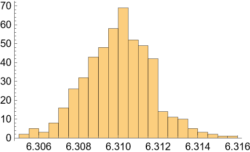 |
Compare with NIntegrate:
| In[110]:= |
| Out[110]= |
Clean up:
| In[111]:= |
Infer the value of an integral from a given set of nodes and function evaluations for the same problem:
| In[112]:= |
| Out[112]= |
| In[113]:= |
| Out[113]= |  |
| In[114]:= | ![nodes = List /@ Subdivide[0., 5., 100];
func = Function[x, Exp[Exp[-x]]];
vals = func[nodes];](https://www.wolframcloud.com/obj/resourcesystem/images/00e/00e34b5b-0d17-4b80-8821-92f7741a4e49/12f9de3396d5ffca.png) |
| In[115]:= |
| Out[115]= |  |
| In[116]:= |
| Out[116]= |  |
| In[117]:= |
| Out[117]= |
Clean up:
| In[118]:= |
Available test problems for probabilistic numerical methods:
| In[119]:= |
| Out[119]= |  |
| In[120]:= |
| Out[120]= |  |
Summary by module:
| In[121]:= | ![Text[Grid[
Prepend[Table[{m, Grid[Module[{o = p[#1]}, {Hyperlink[#1, o["WebInformation"]], o["Information"]["Information"]}] & /@ zoo[m]["Information"]["Functions"], Alignment -> {{Right, Left}, Automatic}]}, {m, zoo["Information"][
"Modules"]}], (Style[#1, Bold] &) /@ {"Module", "Functions"}], Dividers -> Gray, Frame -> Gray, Spacings -> {Automatic, .8}, ItemStyle -> 14]]](https://www.wolframcloud.com/obj/resourcesystem/images/00e/00e34b5b-0d17-4b80-8821-92f7741a4e49/41d981e558ba5540.png) |
| Out[121]= | 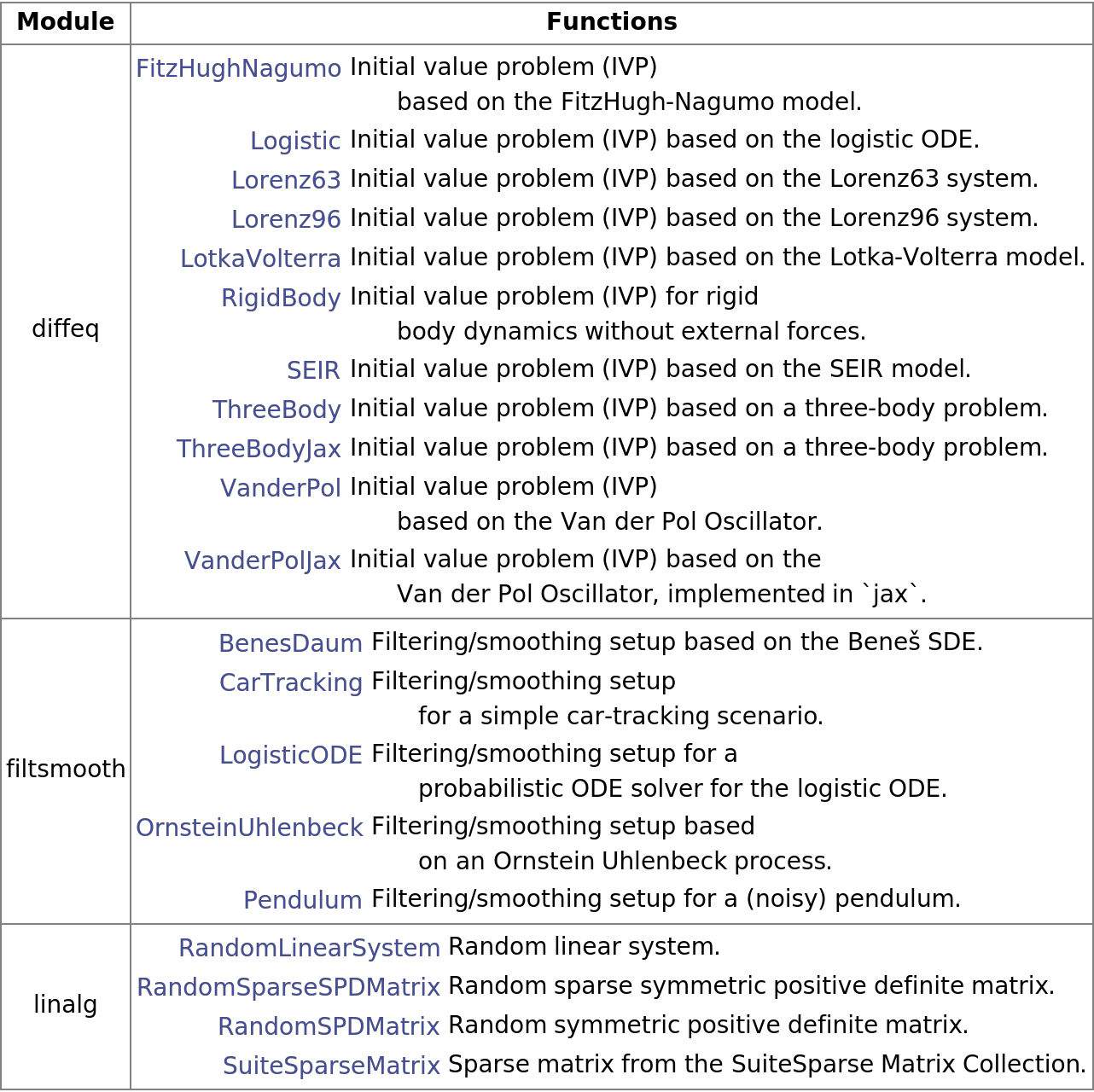 |
| In[122]:= |
Create a FitzHugh-Nagumo model with default parameters:
| In[123]:= |
| Out[123]= |  |
| In[124]:= |
| Out[124]= |  |
Or supply optional parameters:
| In[125]:= |
| Out[125]= |  |
Find solution:
| In[126]:= |
| Out[126]= |  |
Samples from the solution:
| In[127]:= |
| Out[127]= |  |
| In[128]:= |
| Out[128]= | 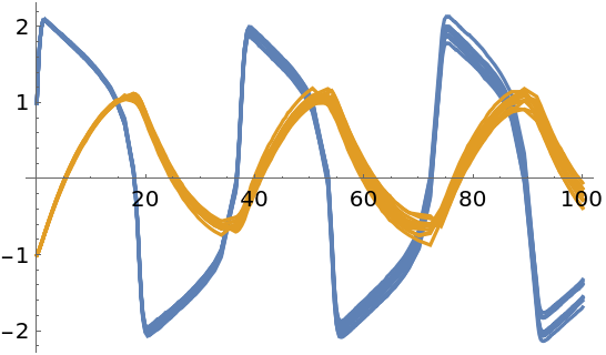 |
Plot together with mean values:
| In[129]:= | ![Show[samples, ResourceFunction["ProbNumObject"]["MeanPlots"[solution]], Frame -> True, FrameLabel -> {"Time", "State variables"}, PlotLabel -> "FitzHugh-Nagumo model"]](https://www.wolframcloud.com/obj/resourcesystem/images/00e/00e34b5b-0d17-4b80-8821-92f7741a4e49/12ce90ff6b4c235b.png) |
| Out[129]= | 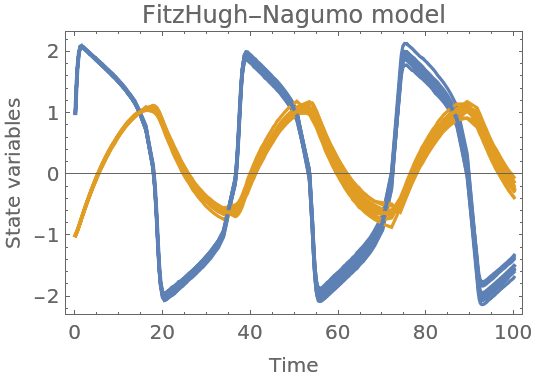 |
| In[130]:= |
Create a model of the Lorenz63 system:
| In[131]:= |
| Out[131]= |  |
| In[132]:= |
| Out[132]= |  |
Find solution of the initial value problem:
| In[133]:= |
| Out[133]= |  |
Plot the mean values:
| In[134]:= |
| Out[134]= | 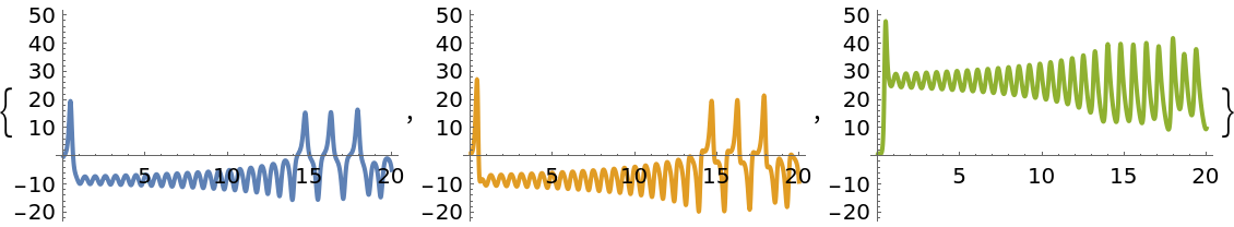 |
Numerical mean values:
| In[135]:= |
| Out[135]= |  |
| In[136]:= |
| Out[136]= |  |
Interpolate mean values:
| In[137]:= |
| Out[137]= |
| In[138]:= |
| Out[138]= | 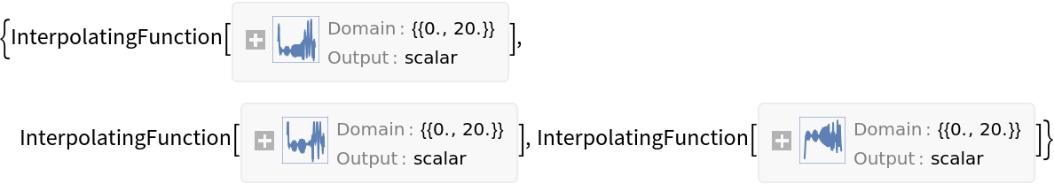 |
| In[139]:= |
| Out[139]= | 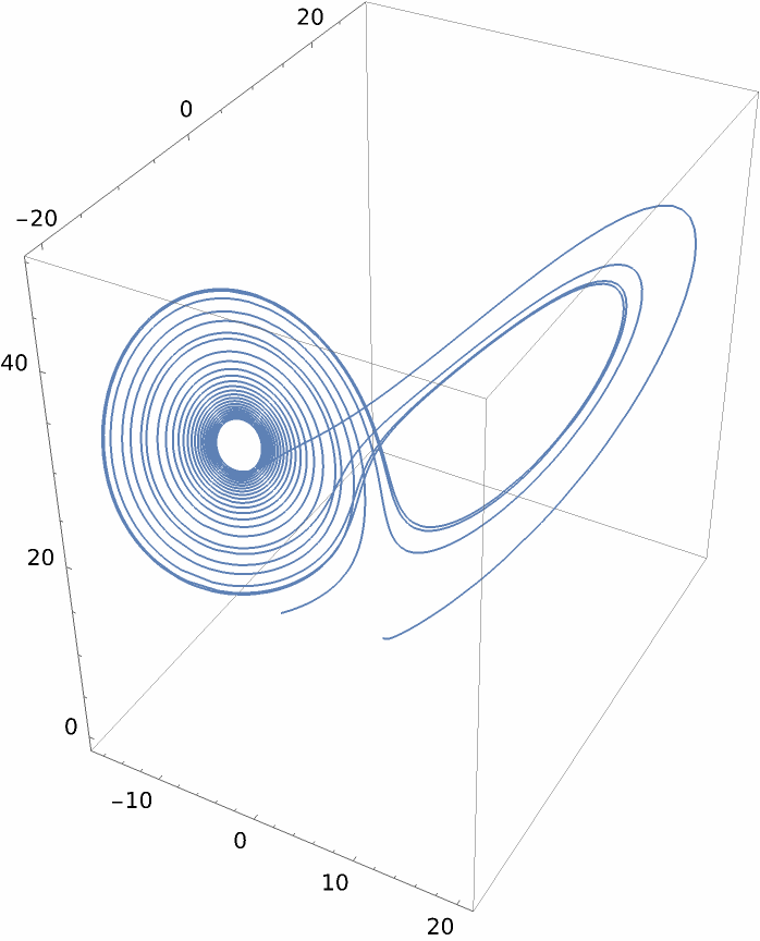 |
| In[140]:= |
Create a random symmetric positive definite matrix:
| In[141]:= |
| Out[141]= |  |
| In[142]:= |
| Out[142]= |  |
| In[143]:= |
| Out[143]= |  |
Convert the object to a list of lists:
| In[144]:= |
| Out[144]= |  |
| Out[124]= |  |
| Out[145]= |  |
Confirm that the matrix has the desired properties:
| In[146]:= |
| Out[146]= |
| In[147]:= |
Create a random symmetric positive definite matrix with a predefined spectrum:
| In[148]:= |
| Out[148]= |  |
| In[149]:= |
| Out[149]= |  |
| In[150]:= |
| In[151]:= |
| Out[151]= |
| In[152]:= |
| Out[152]= |  |
Singular values of the matrix:
| In[153]:= |
| Out[153]= |
| In[154]:= |
| Out[154]= |
| In[155]:= |
Create a sparse random symmetric positive definite matrix:
| In[156]:= |
| Out[156]= |  |
| In[157]:= |
| Out[157]= |  |
| In[158]:= |
| Out[158]= |  |
Convert the Python-side matrix to SparseArray:
| In[159]:= |
| Out[159]= |
| In[160]:= |
| Out[160]= |  |
Confirm that the matrix has the desired properties:
| In[161]:= |
| Out[161]= |
| In[162]:= |
Install the PythonPackage request if it's not installed on your system:
| In[163]:= |
| Out[163]= |
| In[164]:= |
| Out[164]= |
Obtain a sparse matrix from the SuiteSparse Matrix Collection:
| In[165]:= |
| Out[165]= |  |
| In[166]:= |
| Out[166]= |  |
Convert to SparseArray:
| In[167]:= |
| Out[167]= |
| In[168]:= |
| Out[168]= | 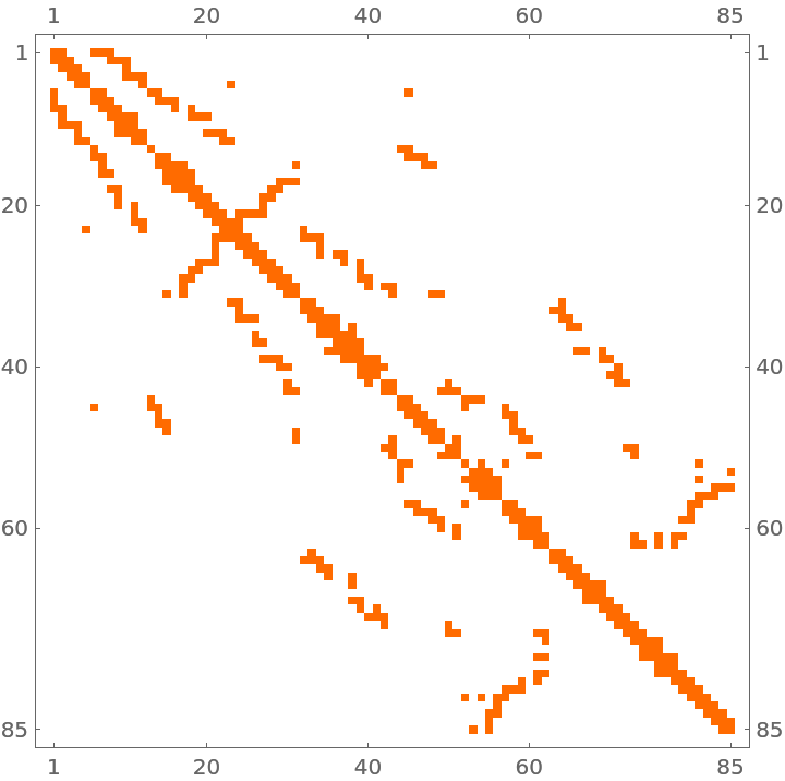 |
Compute the trace of the matrix on the Python side and in the Wolfram Language:
| In[169]:= |
| Out[169]= |
| In[170]:= |
| Out[170]= |
| In[171]:= |
Define a unitary system matrix q:
| In[172]:= | ![n = 5;
a = RandomReal[1, {n, n}];
{q, r} = QRDecomposition[a];
q // TraditionalForm](https://www.wolframcloud.com/obj/resourcesystem/images/00e/00e34b5b-0d17-4b80-8821-92f7741a4e49/67e1bf999f724164.png) |
| Out[129]= |  |
| In[173]:= |
| Out[173]= |
Create a random linear state-space system with the given system matrix:
| In[174]:= |
| Out[174]= |  |
| In[175]:= |
| Out[175]= |  |
| In[176]:= |
| Out[176]= |  |
The component matrices:
| In[177]:= |
| Out[177]= |  |
Convert the Python object to the StateSpaceModel:
| In[178]:= |
| Out[178]= | 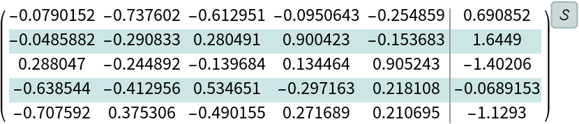 |
| In[179]:= |
Create a linear system with a random symmetric positive-definite matrix:
| In[180]:= |
| Out[180]= |  |
| In[181]:= |
| Out[181]= |  |
| In[182]:= |
| Out[182]= |  |
| In[183]:= |
| Out[183]= |  |
Convert to StateSpaceModel:
| In[184]:= |
| Out[184]= | 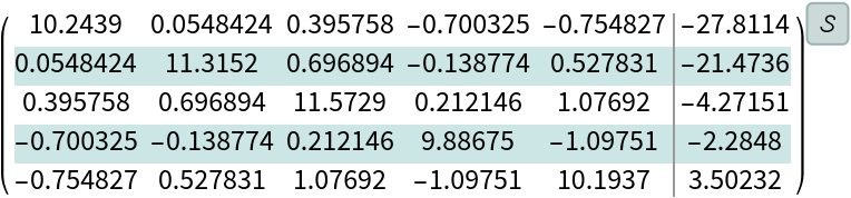 |
| In[185]:= |
Use a sparse random symmetric positive-definite matrix as a system matrix:
| In[186]:= |
| Out[186]= |  |
| In[187]:= |
| Out[187]= |  |
| In[188]:= |
| Out[188]= |  |
| In[189]:= |
| Out[189]= |  |
In the result, the given matrix a is sparse, and the matrix b is dense:
| In[190]:= |
| Out[190]= |
| In[191]:= |
| Out[191]= |
| In[192]:= |
Use Bayesian filtering and smoothing as a framework for efficient inference in state space models:
Model parameters:
| In[193]:= |
Sampling period:
| In[194]:= |
Linear transition operator:
| In[195]:= |
| Out[195]= |  |
Zero-valued force vector for affine transformations of the state:
| In[196]:= |
| Out[196]= |
Covariance matrix of the Gaussian process noise:
| In[197]:= | ![(processNoiseMatrix = DiagonalMatrix[{1/3 deltaT^3, 1/3 deltaT^3, deltaT, deltaT}] + DiagonalMatrix[{deltaT^2/2, deltaT^2/2}, 2] + DiagonalMatrix[{deltaT^2/2, deltaT^2/2}, -2]) // MatrixForm](https://www.wolframcloud.com/obj/resourcesystem/images/00e/00e34b5b-0d17-4b80-8821-92f7741a4e49/5fe09e891957c6ec.png) |
| Out[197]= |  |
Define a linear, time-invariant (LTI) discrete Gaussian state-space dynamics model:
| In[198]:= |
| Out[198]= |  |
| In[199]:= |
| Out[199]= |  |
| In[200]:= |
| Out[200]= |  |
A discrete LTI Gaussian measurement model:
| In[201]:= |
| In[202]:= |
| Out[202]= |
| In[203]:= |
| Out[203]= |
| In[204]:= |
| Out[204]= |  |
| In[205]:= |
| Out[205]= |  |
An initial state random variable:
| In[206]:= |
| Out[206]= |
| In[207]:= |
| Out[207]= |
| In[208]:= |
| Out[208]= |  |
A memoryless prior process:
| In[209]:= |
| Out[209]= |  |
Generate data samples of latent states and noisy observations from the specified state space model:
| In[210]:= |
| In[211]:= |
| Out[211]= |  |
| In[212]:= |
| Out[212]= |  |
| In[213]:= |
| Out[213]= |  |
| In[214]:= |
| Out[214]= |  |
Create a Kalman filter:
| In[215]:= |
| Out[215]= |  |
Perform Kalman Filtering with a Rauch-Tung-Striebel smoothing:
| In[216]:= |
| Out[216]= |  |
| In[217]:= |
| Out[217]= |  |
To visualize the results, prepare plots of mean values from the state posterior object:
| In[218]:= |
Observation plots:
| In[219]:= |
Uncertainty bands:
| In[220]:= |
Combine the plots:
| In[221]:= |
| Out[221]= | 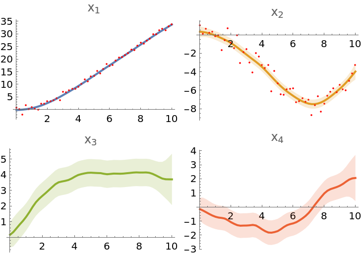 |
| In[222]:= |
Use linearization techniques for Gaussian filtering and smoothing in more complex dynamical systems, such as a pendulum:
Acceleration due to gravity:
| In[223]:= |
Model parameters:
| In[224]:= |
Sampling period:
| In[225]:= |
Define a dynamics transition function and its Jacobian, ignoring the time variable t for time-invariant models:
| In[226]:= |
| In[227]:= |
| Out[227]= |  |
| In[228]:= | ![dynamicsTransitionFunction = ResourceFunction["ToPythonFunction"][session, Function[{t, state}, {x1 + x2*deltaT, x2 - g*Sin[x1]*deltaT}] /. {x1 :> state[[1]], x2 :> state[[2]]}, Method -> "np"]](https://www.wolframcloud.com/obj/resourcesystem/images/00e/00e34b5b-0d17-4b80-8821-92f7741a4e49/2d4df84c68083e38.png) |
| Out[228]= | 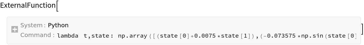 |
| In[229]:= | ![dynamicsTransitionJacobianFunction = ResourceFunction["ToPythonFunction"][session, Function[{t, state}, {{1, deltaT}, {-g * Cos[x1] * deltaT, 1.}}] /. {x1 :> state[[1]], x2 :> state[[2]]}, Method -> "np"]](https://www.wolframcloud.com/obj/resourcesystem/images/00e/00e34b5b-0d17-4b80-8821-92f7741a4e49/1f9014869b16bd03.png) |
| Out[229]= | 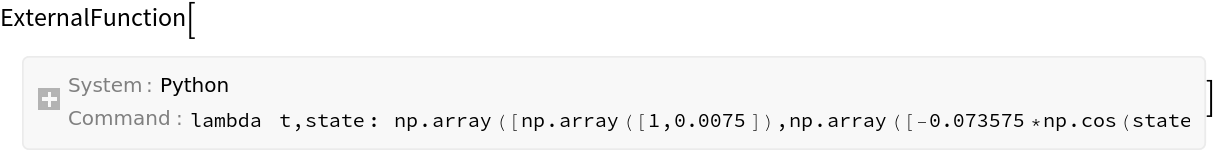 |
Diffusion matrix:
| In[230]:= | ![dynamicsDiffusionMatrix = DiagonalMatrix[{deltaT^3/3, deltaT}] + DiagonalMatrix[{deltaT^2/2}, 1] + DiagonalMatrix[{deltaT^2/2}, -1]](https://www.wolframcloud.com/obj/resourcesystem/images/00e/00e34b5b-0d17-4b80-8821-92f7741a4e49/1757fe4998ca673f.png) |
| Out[230]= |
| In[231]:= |
| Out[231]= |  |
| In[232]:= |
| Out[232]= |
Create a discrete, non-linear Gaussian dynamics model:
| In[233]:= | ![dynamicsModel = p["NonlinearGaussian"["InputDim" -> stateDimensions, "OutputDim" -> stateDimensions, "TransitionFunction" -> dynamicsTransitionFunction, "NoiseFunction" -> noiseFunction, "TransitionFunctionJacobian" -> dynamicsTransitionJacobianFunction]]](https://www.wolframcloud.com/obj/resourcesystem/images/00e/00e34b5b-0d17-4b80-8821-92f7741a4e49/50e196c56ec2384f.png) |
| Out[233]= |  |
Prepare functions that define nonlinear Gaussian measurements:
| In[234]:= |
| Out[234]= |
| In[235]:= | ![measurementJacobianFunction = ResourceFunction["ToPythonFunction"][session, Function[{t, state}, {{Cos[state[[1]]], 0.}}], Method -> "np"]](https://www.wolframcloud.com/obj/resourcesystem/images/00e/00e34b5b-0d17-4b80-8821-92f7741a4e49/0ee1130992225965.png) |
| Out[235]= |
| In[236]:= |
| Out[236]= |
| In[237]:= |
| Out[237]= |
| In[238]:= |
| Out[238]= |  |
| In[239]:= |
| Out[239]= |
Create discrete, non-linear Gaussian measurement model:
| In[240]:= | ![measurementModel = p["NonlinearGaussian"["InputDim" -> stateDimensions, "OutputDim" -> observationDimensions, "TransitionFunction" -> measurementFunction, "NoiseFunction" -> measurementNoiseFunction, "TransitionFunctionJacobian" -> measurementJacobianFunction]]](https://www.wolframcloud.com/obj/resourcesystem/images/00e/00e34b5b-0d17-4b80-8821-92f7741a4e49/1a6d291655f6ecd9.png) |
| Out[240]= |  |
Initial state random variable:
| In[241]:= |
| Out[241]= |
| In[242]:= |
| Out[242]= |
| In[243]:= |
| Out[243]= |  |
Linearize the model to create the Extended Kalman Filter (EKF):
| In[244]:= |
| Out[244]= |  |
| In[245]:= |
| Out[245]= |  |
| In[246]:= |
| Out[246]= |  |
Generate data for the state-space model:
| In[247]:= |
| In[248]:= |
| Out[248]= |  |
| In[249]:= |
| Out[249]= |  |
| In[250]:= |
| Out[250]= |  |
| In[251]:= | ![regressionProblem = p["TimeSeriesRegressionProblem"[timeGrid, observations, p["DiscreteEKFComponent"[measurementModel]]]]](https://www.wolframcloud.com/obj/resourcesystem/images/00e/00e34b5b-0d17-4b80-8821-92f7741a4e49/730ebe066989dcd7.png) |
| Out[251]= |  |
Perform Kalman filtering with Rauch-Tung-Striebel smoothing:
| In[252]:= |
| Out[252]= |  |
| In[253]:= |
| Out[253]= | 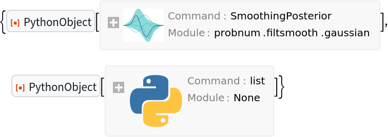 |
Prepare mean value plots of the state posterior object:
| In[254]:= |
Display a few samples from the state posterior on a subsampled grid, taking every fifth point for clarity:
| In[255]:= |
| Out[255]= | 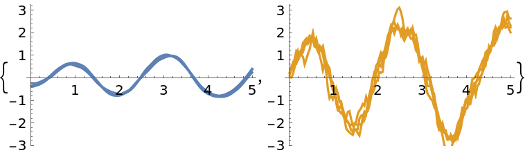 |
Prepare plots of uncertainty bands:
| In[256]:= |
Observations:
| In[257]:= |
Combine the plots:
| In[258]:= |
| Out[258]= | 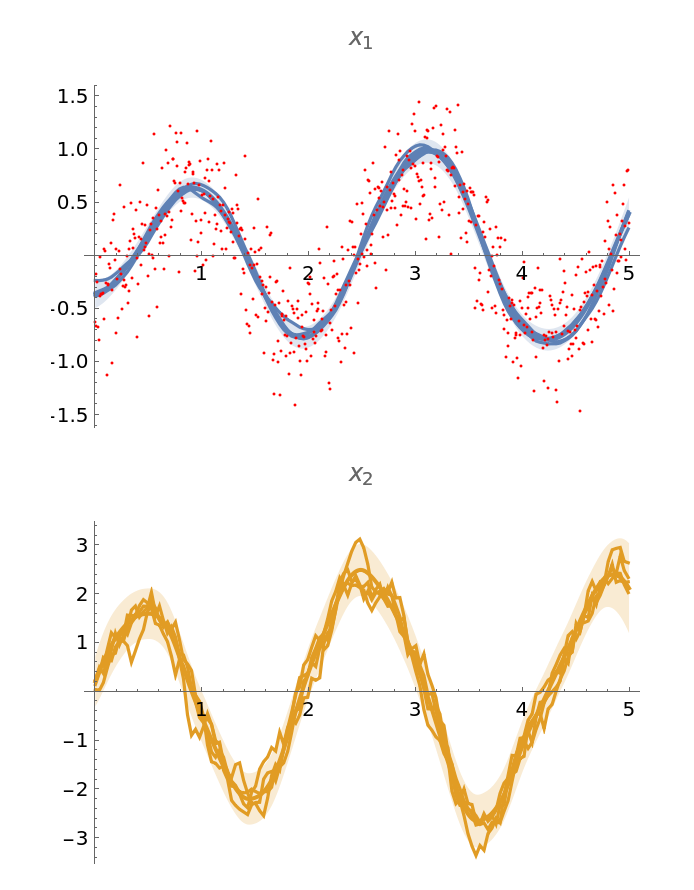 |
| In[259]:= |
Use a set of particles (samples) to represent the posterior distribution of a stochastic process given noisy observations.
Create a pendulum model from scratch, as in the Nonlinear Gaussian Filtering and Smoothing example, or use a predefined test problem:
| In[260]:= |
| Out[260]= |  |
| In[261]:= |
| Out[261]= |  |
| In[262]:= | ![{regressionProblem, rpInfo} = Normal@p[
"Pendulum"[rng, "MeasurementVariance" -> 0.12^2, "Timespan" -> {0, 3.5}, "Step" -> 0.05]]](https://www.wolframcloud.com/obj/resourcesystem/images/00e/00e34b5b-0d17-4b80-8821-92f7741a4e49/611bdbeeab3c7c42.png) |
| Out[262]= |  |
Extract parameters needed to set up a particle filer, starting from the prior process:
| In[263]:= |
| Out[263]= |  |
| In[264]:= |
| Out[264]= |  |
Also get the dynamics model and the measurement model:
| In[265]:= |
| Out[265]= |  |
| In[266]:= |
| Out[266]= |  |
Create a linearized the importance distribution from the extended Kalman filer:
| In[267]:= |
| Out[267]= |  |
| In[268]:= |
| Out[268]= |  |
Define the number of particles:
| In[269]:= |
Create a particle filter:
| In[270]:= |
| Out[270]= |  |
Apply the filter and obtain the posterior distribution:
| In[271]:= |
| Out[271]= |  |
| In[272]:= |
| Out[272]= |  |
The states of posterior:
| In[273]:= |
| Out[273]= |  |
Plot the latent state together with the mode of the posterior distribution:
| In[274]:= |
| In[275]:= |
| In[276]:= |
| In[277]:= |
| In[278]:= |
| Out[278]= | 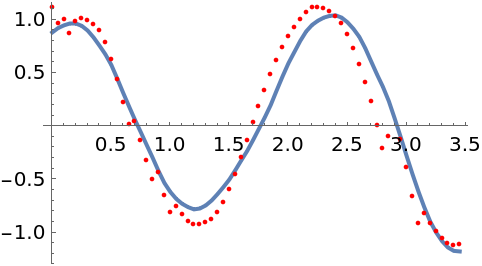 |
The true latent state is recovered fairly well. The root-mean-square error (RNSE) of the mode is also much smaller than the RMSE of the data:
| In[279]:= |
| Out[279]= |
| In[280]:= |
| In[281]:= |
| Out[281]= |
Plot a few more particles, removing the unlikely ones by resampling the posterior. The distribution concentrates around the true state:
| In[282]:= |
| Out[282]= |  |
| In[283]:= | ![Show[lsplot, Table[ListPlot[
Transpose[{locations, Normal[resampledStates["support"] // Normal][[All, i, 1]]}], PlotStyle -> Orange], {i, numParticles}], Frame -> True, GridLines -> Automatic]](https://www.wolframcloud.com/obj/resourcesystem/images/00e/00e34b5b-0d17-4b80-8821-92f7741a4e49/2fd2831ff93be999.png) |
| Out[283]= | 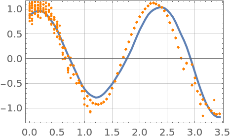 |
| In[284]:= |
Set up a Bernoulli equation and its Jacobian:
| In[285]:= |
| Out[285]= |
| In[286]:= |
| Out[286]= |
| In[287]:= | ![bernJac = ResourceFunction["ToPythonFunction"][session, Function[{t, x}, {1.5 (1 - 3 x^2)}], Epilog -> "np.array"]](https://www.wolframcloud.com/obj/resourcesystem/images/00e/00e34b5b-0d17-4b80-8821-92f7741a4e49/573d930dd4b6610f.png) |
| Out[287]= |
Construct an initial value problem:
| In[288]:= |
| Out[288]= |  |
| In[289]:= |
| In[290]:= |
| Out[290]= |  |
Use integrator as a dynamics model:
| In[291]:= |
| Out[291]= |  |
Add a small “evaluation variance" to the initial random variable:
| In[292]:= |
| In[293]:= |
| Out[293]= |  |
| In[294]:= |
| Out[294]= |  |
Construct an importance distribution using the extended Kalman filter:
| In[295]:= |
| Out[295]= |  |
| In[296]:= | ![importance = fromEKF[All][dynamicsModel, "BackwardImplementation" -> "sqrt", "ForwardImplementation" -> "sqrt"]](https://www.wolframcloud.com/obj/resourcesystem/images/00e/00e34b5b-0d17-4b80-8821-92f7741a4e49/6b5c85951e049a5c.png) |
| Out[296]= |  |
Create a particle filter:
| In[297]:= |
| In[298]:= |
| Out[298]= |  |
| In[299]:= |
| Out[299]= |  |
Define a grid of evenly spaced points:
| In[300]:= |
| In[301]:= |
Information operator that measures the residual of an explicit ODE:
| In[302]:= |
| Out[302]= |  |
Make inference with an information operator using a first-order linearization of the ODE vector-field:
| In[303]:= |
| Out[303]= |  |
Define a regression problem:
| In[304]:= | ![regressionProblem = p["IVPToRegressionProblem"[
bernoulli,
locations,
infoOp,
"ApproximateStrategy" -> ek1,
"ExcludeInitialCondition" -> True,
"ODEMeasurementVariance" -> 0.00001
]]](https://www.wolframcloud.com/obj/resourcesystem/images/00e/00e34b5b-0d17-4b80-8821-92f7741a4e49/59fce5ca03c039c0.png) |
| Out[304]= |  |
Find the ODE posterior:
| In[305]:= |
| Out[305]= |  |
| In[306]:= |
| Out[306]= |  |
Resample removing the unlikely particles:
| In[307]:= |
| Out[307]= |  |
Plot the solution. Depending on the position of the initial particle, the trajectories deviate from the unstable equilibrium at 0 and approach either of the stable equilibria, +1 or -1:
| In[308]:= |
| Out[308]= | 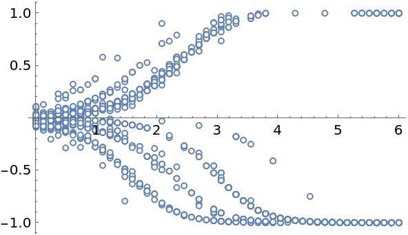 |
For comparison, solve the equation with DSolve:
| In[309]:= |
| Out[309]= |
| In[310]:= |
| Out[310]= | 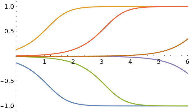 |
| In[311]:= |
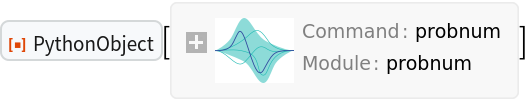
ProbNumObject[…] gives the same result as the resource function PythonObject with a special configuration:
| In[312]:= |
| Out[312]= |
| In[313]:= |
| Out[313]= |  |
| In[314]:= |
| Out[314]= |  |
| In[315]:= |
Available functions:
| In[316]:= |
| Out[316]= |  |
| In[317]:= |
| Out[317]= |  |
Information on a function:
| In[318]:= |
| Out[318]= |  |
Search the web documentation for a function in your default browser:
| In[319]:= |
| In[320]:= |
Find a Wolfram language name for a Python-side function:
| In[321]:= |
| Out[321]= |  |
| In[322]:= |
| Out[322]= |
Or a Python name corresponding to a Wolfram-Language name:
| In[323]:= |
| Out[323]= |
The list of conversion rules:
| In[324]:= |
| Out[324]= |
| In[325]:= |
Solve a linear matrix equation with LinearSolve:
| In[326]:= |
| In[327]:= |
| Out[327]= |
Solve the same equation with ProbNum:
| In[328]:= |
| Out[328]= |  |
| In[329]:= |
| Out[329]= |  |
The multivariate Gaussian random variable corresponding to the solution:
| In[330]:= |
| Out[330]= |  |
The mean of the normal distribution equals the best guess for the solution of the linear system:
| In[331]:= |
| Out[331]= |
| In[332]:= |
| Out[332]= |
The covariance matrix provides a measure of uncertainty:
| In[333]:= |
| Out[333]= |
In this case, the algorithm is very certain about the solution as the covariance matrix is virtually zero:
| In[334]:= |
| Out[334]= |
Clean up by closing the Python session:
| In[335]:= |
Display the first few matrices from the SuiteSparse Matrix Collection:
| In[336]:= |
| Out[336]= |  |
| In[337]:= |
Install the requests module, if it's not yet installed in your Python:
| In[338]:= |
| Out[338]= |
| In[339]:= |
| In[340]:= | ![Text@Grid[
Prepend[data /. sp_SparseArray :> MatrixPlot[sp], {"ID", "Name", "Group", "Kind", "Shape", ""}], Background -> {None, {Lighter[Yellow, .5], {White, Lighter[LightGreen, .5]}}}, Dividers -> Gray, ItemSize -> {{3, 7, 5, 10}}, Frame -> Gray, Spacings -> {Automatic, .8}, ItemStyle -> 14]](https://www.wolframcloud.com/obj/resourcesystem/images/00e/00e34b5b-0d17-4b80-8821-92f7741a4e49/35f9514fafec9330.png) |
| Out[340]= | 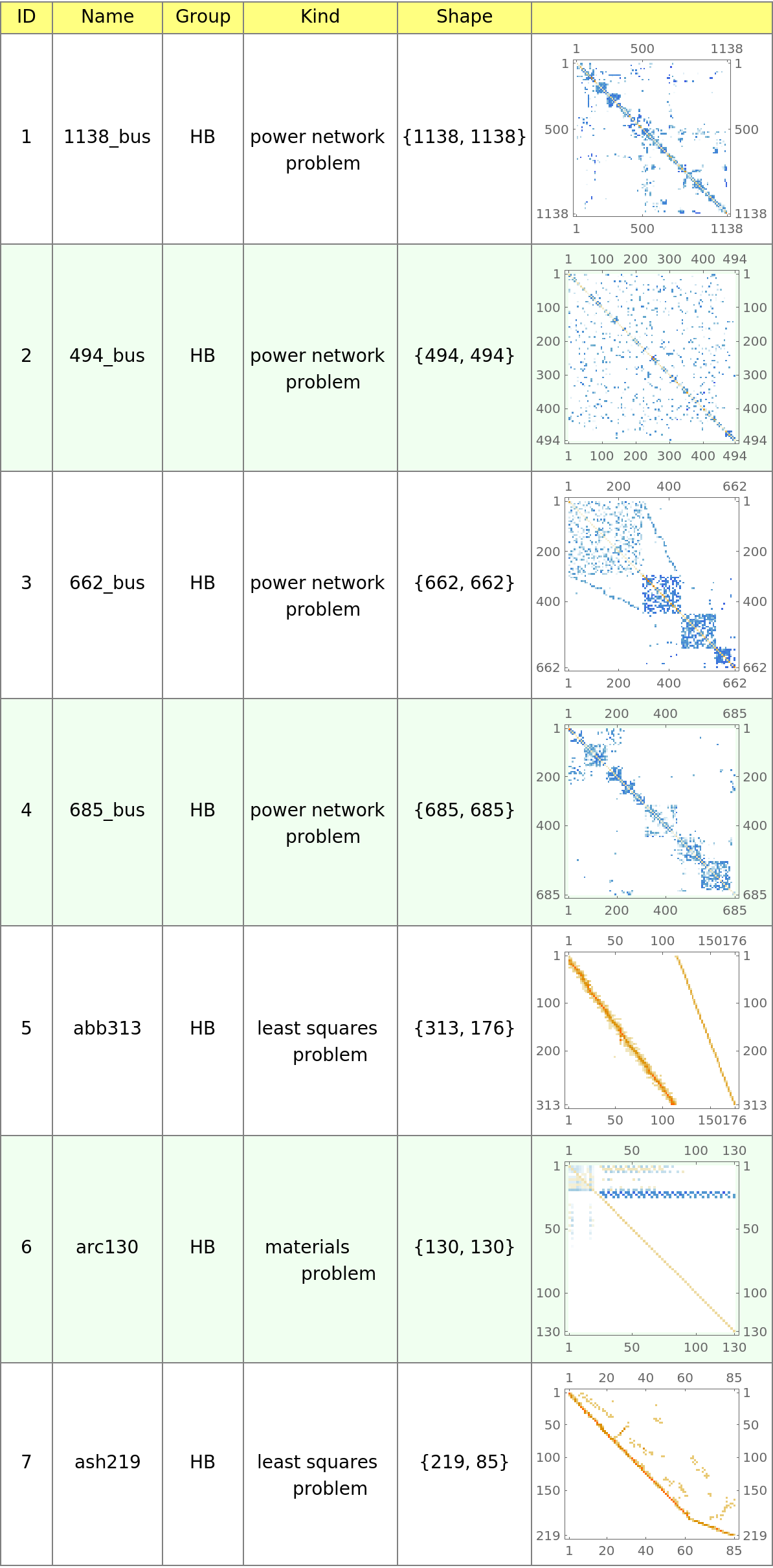 |
| In[341]:= |
Signatures of LTIGaussian and NonlinearGaussian changed in ProbNum v. 0.1.17. If the related examples in the Applications section fail for you with:
… update your ProbNum to a more recent version. To check the version:
| In[1]:= |
| In[2]:= |
| In[3]:= |
This work is licensed under a Creative Commons Attribution 4.0 International License