Wolfram Function Repository
Instant-use add-on functions for the Wolfram Language
Function Repository Resource:
Approximate a function with a polynomial
ResourceFunction["PolynomialApproximation"][f,{x,xmin,xmax},n, "type"] finds an nth order polynomial of a given type that approximates the function f for x∈[xmin,xmax]. |
| "Taylor" | Taylor expansion around (xmin+xmax)/2 |
| "Equispaced" | Polynomial going through n+1 points equispaced between xmin and xmax |
| "Chebyshev" | Polynomial going through n+1 Chebyshev nodes |
| "Remez" | Iteratively optimize the nodes starting with Chebyshev nodes |
| {“Remez”, m} | Remez with m iterations |
Find the second-order Taylor polynomial approximating the sine function:
| In[1]:= |
| Out[1]= |
Compare with the original function:
| In[2]:= |
| Out[2]= | 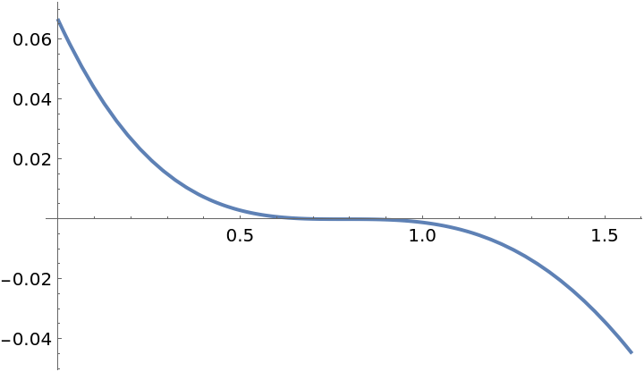 |
Use equispaced points to get a better approximation:
| In[3]:= | ![f = Sin[x];
g = ResourceFunction["PolynomialApproximation"][f, {x, 0.0, Pi/2}, 2, "Equispaced"];
Plot[f - g, {x, 0, Pi/2}]](https://www.wolframcloud.com/obj/resourcesystem/images/bd1/bd1baeab-64a2-4884-9f2f-5bd99a8d1103/06841eb033211ec6.png) |
| Out[5]= | 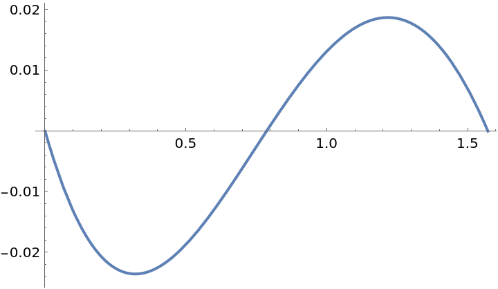 |
Use Chebyshev points to get an even better approximation:
| In[6]:= | ![f = Sin[x];
g = ResourceFunction["PolynomialApproximation"][f, {x, 0.0, Pi/2}, 2, "Chebyshev"];
Plot[f - g, {x, 0, Pi/2}]](https://www.wolframcloud.com/obj/resourcesystem/images/bd1/bd1baeab-64a2-4884-9f2f-5bd99a8d1103/20574816367dde02.png) |
| Out[8]= | 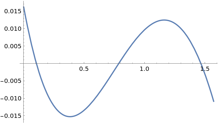 |
The polynomial produced by the Remez method yields a nearly-optimal approximation:
| In[9]:= | ![f = Sin[x];
g = ResourceFunction["PolynomialApproximation"][f, {x, 0.0, Pi/2}, 2, "Remez"];
Plot[f - g, {x, 0, Pi/2}]](https://www.wolframcloud.com/obj/resourcesystem/images/bd1/bd1baeab-64a2-4884-9f2f-5bd99a8d1103/4c874c94cec9c325.png) |
| Out[11]= | 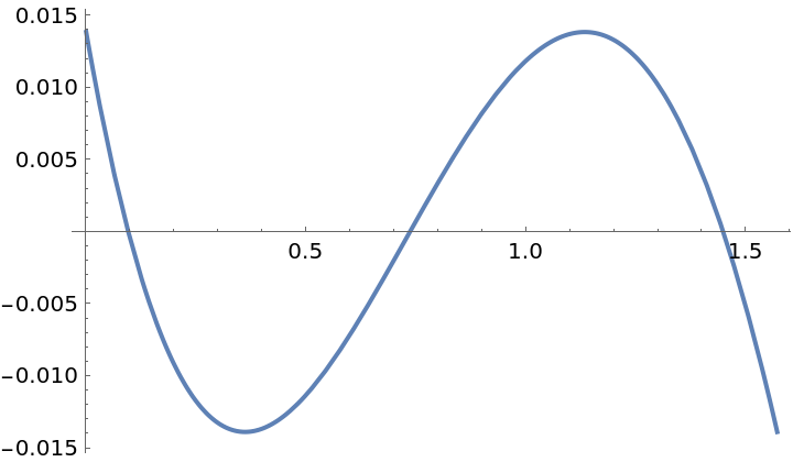 |
Perform 6 iterations for the Remez method, and then compare the error:
| In[12]:= | ![f = BesselJ[0, x];
g = ResourceFunction["PolynomialApproximation"][f, {x, 0.0, 3}, 5, {"Remez", 6}];
Plot[f - g, {x, 0, 3}]](https://www.wolframcloud.com/obj/resourcesystem/images/bd1/bd1baeab-64a2-4884-9f2f-5bd99a8d1103/2eaf710be352661f.png) |
| Out[14]= | 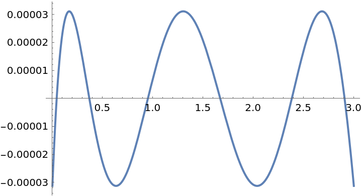 |
Find a function that can approximate the cosine function for angles up to ![]() :
:
| In[15]:= |
| Out[16]= | 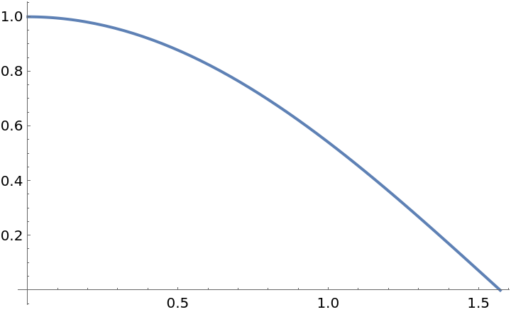 |
Calculate several orders and compare the maximum absolute error:
| In[17]:= | ![gs = Table[
ResourceFunction["PolynomialApproximation"][f, {x, 0.0, Pi/2}, n, {"Remez", 8}]
,
{n, 2, 7}
];
LogPlot[Evaluate[Abs[(f - #)] & /@ gs], {x, 0, Pi/2}, PlotRange -> All, PlotLegends -> Range[2, 7], Frame -> True, PlotRangePadding -> {Scaled[.01], Scaled[.12]}, Axes -> False, PerformanceGoal -> "Speed"]](https://www.wolframcloud.com/obj/resourcesystem/images/bd1/bd1baeab-64a2-4884-9f2f-5bd99a8d1103/2b41169b8b48b785.png) |
| Out[18]= | 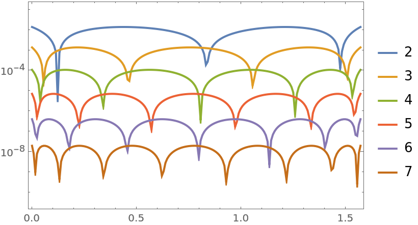 |
The Remez method does not always converge:
| In[19]:= | ![f = Cos[x];
g = ResourceFunction["PolynomialApproximation"][f, {x, 0.0, 3.0}, 3, {"Remez", 10}];
Plot[f - g, {x, 0, 3}]](https://www.wolframcloud.com/obj/resourcesystem/images/bd1/bd1baeab-64a2-4884-9f2f-5bd99a8d1103/003493844e01b3c4.png) |
| Out[21]= |  |
Higher order Remez might not converge to a good solution:
| In[22]:= | ![f = Cos[x];
g = ResourceFunction["PolynomialApproximation"][f, {x, 0.0, 3}, 12, {"Remez", 20}];
Plot[f - g, {x, 0, 3}]](https://www.wolframcloud.com/obj/resourcesystem/images/bd1/bd1baeab-64a2-4884-9f2f-5bd99a8d1103/79180da560e387c5.png) |
| Out[24]= | 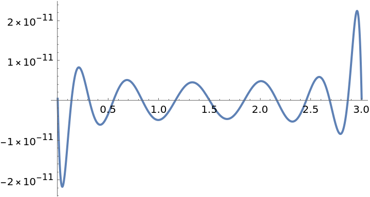 |
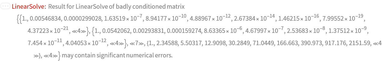
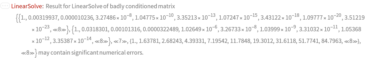
Higher order Remez might be prone to numerical errors:
| In[25]:= |
| Out[25]= |  |
Functions that are not continuous can not be approximated very well:
| In[26]:= | ![f = 1/(x - 1);
g = ResourceFunction["PolynomialApproximation"][1/(
x - 1), {x, 0.0, 3}, 5, "Equispaced"];
Plot[{f, g}, {x, 0, 3}]](https://www.wolframcloud.com/obj/resourcesystem/images/bd1/bd1baeab-64a2-4884-9f2f-5bd99a8d1103/742847b99fc9ee6e.png) |
| Out[28]= | 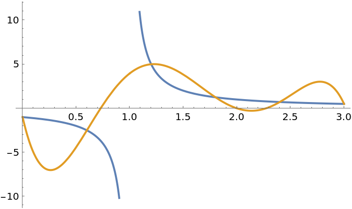 |
Find a function that approximates a normal distribution:
| In[29]:= | ![f = Exp[-x^2];
g = Quiet@
ResourceFunction["PolynomialApproximation"][f, {x, 0.0, 4}, 12, {"Remez", 8}];
Plot[f - g, {x, 0, 4}]](https://www.wolframcloud.com/obj/resourcesystem/images/bd1/bd1baeab-64a2-4884-9f2f-5bd99a8d1103/67c6751962421589.png) |
| Out[31]= | 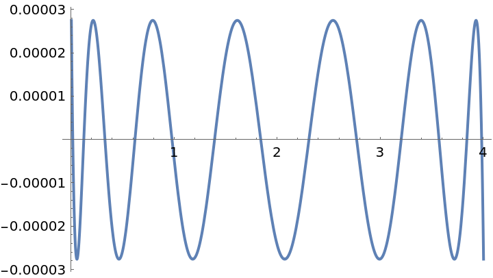 |
Find the maximum error:
| In[32]:= |
| Out[32]= |
Compare that to the Chebyshev case:
| In[33]:= | ![f = Exp[-x^2];
g = Quiet@
ResourceFunction["PolynomialApproximation"][f, {x, 0.0, 4}, 12, "Chebyshev"];
Plot[f - g, {x, 0, 4}]](https://www.wolframcloud.com/obj/resourcesystem/images/bd1/bd1baeab-64a2-4884-9f2f-5bd99a8d1103/77863ecc75d93e12.png) |
| Out[34]= | 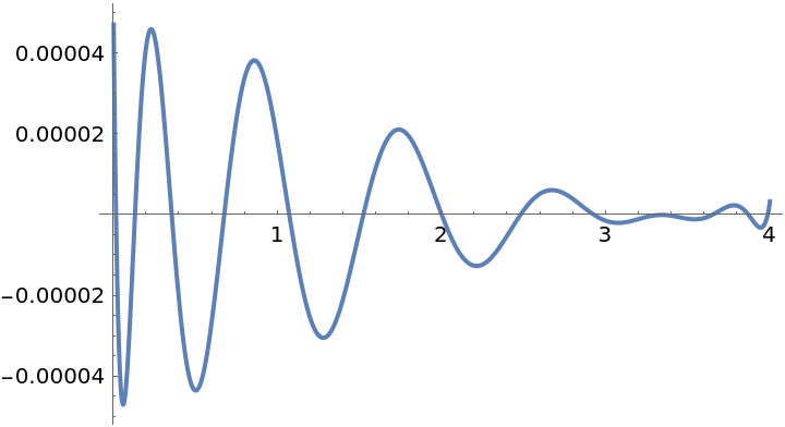 |
| In[35]:= |
| Out[35]= |
Wolfram Language 13.2 (December 2022) or above
This work is licensed under a Creative Commons Attribution 4.0 International License