Details
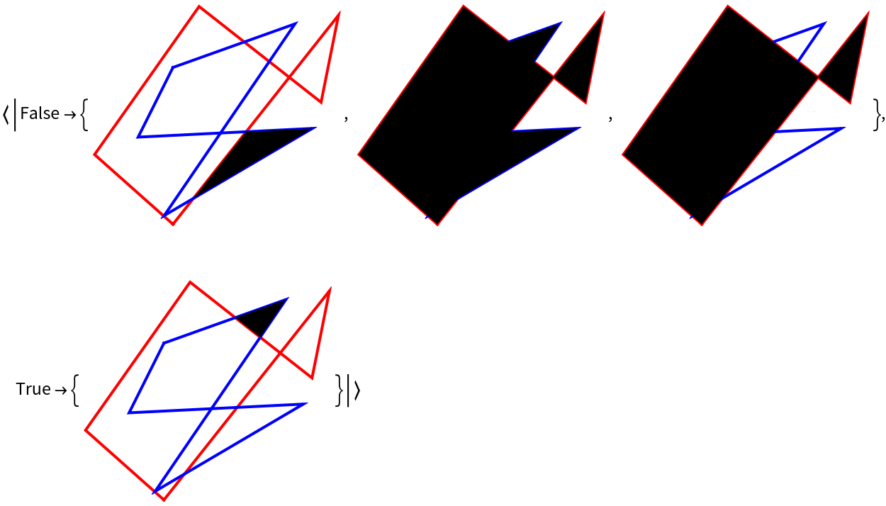
To fragment polygons p1 and p2, we join their combined edge and vertex sets, adding new vertices wherever an edge of p1 crosses an edge of p2. The new set of edges and vertices bounds a finite set of simple polygons (i.e. topological disks), also called “fragments” of p1 and p2.
Fragments are extracted and returned in two classes. One class contains the intersection(s) and union of p1 and p2, while the other contains the pairwise complements between p1 and p2.
If the vertices of
p1 and
p2, have the same circularity (or handedness), then the intersection/union class falls under the
True key, while differences fall under the
False key.
If the circularity of
p1 and
p2 are opposite, then the
True/
False keys are transposed.
There are several polygon clipping algorithms. Transposition for opposite-handedness is consistent with set operations when considering circularity as the determining measure of whether the polygon's filled area is either interior or exterior to the boundary. Such a convention is relatively common in high-power clipping algorithms, and it is also a feature of the wedge product in symplectic geometry.
If the combination of
p1 and
p2 encloses a polygonal hole, it will become a fragment in the same class as the intersection(s). In this case the union needs a more complicated form,
Polygon[
frag1→
frag2], where
frag1 and
frag2 are outer and inner boundaries respectively. Considering the outer boundary as enclosing the figure's exterior (including the point at infinity), the union of all fragments should be an exact cover of the entire plane.
ResourceFunction["PlanarPolygonFragmentation"] takes one option "BinCount" →
n, with default value
n = 1. When
n is set to a positive integer greater than 1, the input vertices and edges are discretized into approximately
n2 bins, which allows intersections to be solved locally. For polygons with many edge segments, this saves considerable time by avoiding unnecessary, brute force calculation via
Outer. This improves speed, but in pathological cases can lead to incorrect results.
Even in cases where discretization is necessary, a law of diminishing returns applies. There is usually a best choice for "BinCount", which may require experimentation or heuristics to find. In the case of inputs with few edges, setting "BinCount" greater than 1 is not necessary.
Self-intersecting polygons and polygons with holes are not valid inputs. Should one desire, they can be broken up into lists of simple polygons, which can then be folded through the fragmentation process.
ResourceFunction["PlanarPolygonFragmentation"] can be used to solve planar clipping problems. Our algorithm is already more powerful and can be faster than the numerical standard Greiner-Hormann. In utilizing discrete methods,
ResourceFunction["PlanarPolygonFragmentation"] goes below the naive order
O(n*m) complexity limit, which was carried through the subsequent work "Clipping simple polygons with degenerate intersections" (see references below).
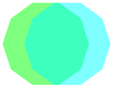
![{p1, p2} = {
Polygon[CirclePoints[{0, 0}, {1, 0}, 10]],
Polygon[CirclePoints[{1/2, 0}, {1, 0}, 10]]
};
Graphics[{Opacity[.5], Green, p1, Cyan, p2}]](https://www.wolframcloud.com/obj/resourcesystem/images/b75/b75682f5-b29f-4b24-8ecd-41055888a8f4/3da80b4ade3bf4e0.png)

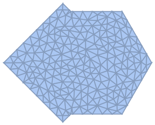
![ResourceFunction["PlanarPolygonFragmentation"][
Polygon[{{1, 1}, {-1, 1}, {-1, -1}, {1, -1}}],
Polygon[{{1, 1}, {1/2, 3/2}, {0, 1}, {1/2, 1/2}}]
]](https://www.wolframcloud.com/obj/resourcesystem/images/b75/b75682f5-b29f-4b24-8ecd-41055888a8f4/4655f8c276fb7d1c.png)

![res = ResourceFunction["PlanarPolygonFragmentation"][
Polygon[CirclePoints[{0, 0}, {1/2, Pi/6}, 6]],
Polygon[CirclePoints[{Sqrt[3]/2, 1/5}, {1/2, Pi/6}, 6]]
]](https://www.wolframcloud.com/obj/resourcesystem/images/b75/b75682f5-b29f-4b24-8ecd-41055888a8f4/32a54d08e2d40fbb.png)


![ResourceFunction["PlanarPolygonFragmentation"][
Polygon[CirclePoints[{0, 0}, {1/2, Pi/6}, 6], Range[6]],
Polygon[CirclePoints[{1/2, 0}, {1/2, 2 Pi/5}, 4], Range[4]]
]](https://www.wolframcloud.com/obj/resourcesystem/images/b75/b75682f5-b29f-4b24-8ecd-41055888a8f4/09a1e80635153fed.png)


![AbsoluteTiming[
With[{res = ResourceFunction["PlanarPolygonFragmentation"][
franceMainland, cutWith, "BinCount" -> 100]},
Graphics@res[True][[2]]
]]](https://www.wolframcloud.com/obj/resourcesystem/images/b75/b75682f5-b29f-4b24-8ecd-41055888a8f4/4d8c21a74ee4796d.png)

![AbsoluteTiming[
With[{res = ResourceFunction["PlanarPolygonFragmentation"][
franceMainland, cutWith, "BinCount" -> 1000]},
Graphics@res[True][[2]]
]
]](https://www.wolframcloud.com/obj/resourcesystem/images/b75/b75682f5-b29f-4b24-8ecd-41055888a8f4/3e906b828138f1a3.png)

![p1 = ReverseSortBy[ResourceFunction["PlanarPolygonFragmentation"][
Polygon[CirclePoints[{0, 0}, {1, 0}, 4]],
Polygon[CirclePoints[{1/2, 0}, {1, 0}, 6]]
][True], Area, NumericalOrder][[1]]](https://www.wolframcloud.com/obj/resourcesystem/images/b75/b75682f5-b29f-4b24-8ecd-41055888a8f4/01ecc4f2b72bd86d.png)
![AbsoluteTiming[
res1 = ReverseSortBy[ResourceFunction["PlanarPolygonFragmentation"][
Polygon[CirclePoints[{0, 0}, {1, 0}, 5]],
Polygon[CirclePoints[{1/2, 0}, {1, 0}, 6]]
][True], Area, NumericalOrder][[2]]]](https://www.wolframcloud.com/obj/resourcesystem/images/b75/b75682f5-b29f-4b24-8ecd-41055888a8f4/6a6f8d688e053a1a.png)
![AbsoluteTiming[
res2 = RegionIntersection[Polygon[CirclePoints[{0, 0}, {1, 0}, 5]],
Polygon[CirclePoints[{1/2, 0}, {1, 0}, 6]]]
]](https://www.wolframcloud.com/obj/resourcesystem/images/b75/b75682f5-b29f-4b24-8ecd-41055888a8f4/02322d82a1842ca2.png)
![AbsoluteTiming[
First[With[{p1 = Polygon[CirclePoints[{0, 0}, {1, 0}, 4]]},
Select[ResourceFunction["PlanarPolygonFragmentation"][p1,
Polygon[CirclePoints[{1/2, 0}, {1, 0}, 6]]
][False], RegionMember[p1,
RandomPoint[#]] &
]]]
]](https://www.wolframcloud.com/obj/resourcesystem/images/b75/b75682f5-b29f-4b24-8ecd-41055888a8f4/1087069990250f2a.png)
![AbsoluteTiming[
RegionDifference[Polygon[CirclePoints[{0, 0}, {1, 0}, 5]],
Polygon[CirclePoints[{1/2, 0}, {1, 0}, 6]]]
]](https://www.wolframcloud.com/obj/resourcesystem/images/b75/b75682f5-b29f-4b24-8ecd-41055888a8f4/2dc5e557887005d1.png)

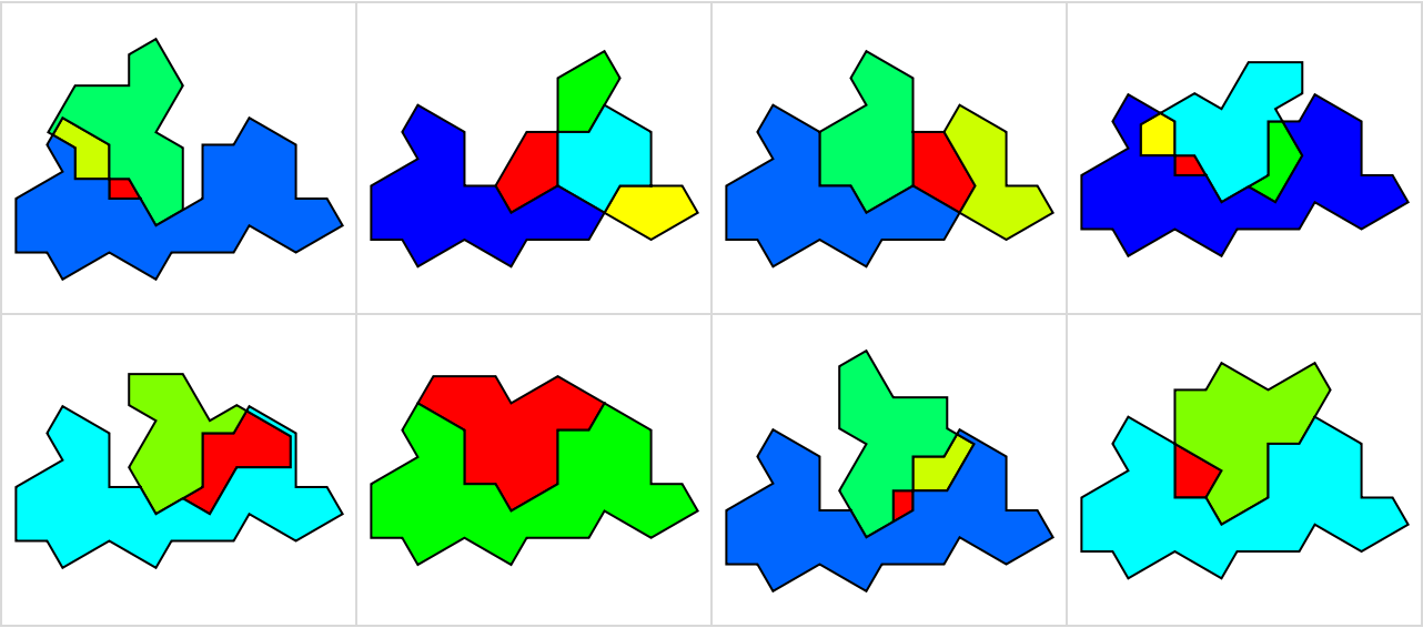
![polys = With[{
rand = SeedRandom[123],
vertices = Divide[RandomInteger[{0, 100}, {2, 10, 2}], 100]},
Map[Polygon[#[[Drop[Last[FindShortestTour[#]], -1]]]] &,
vertices]
];](https://www.wolframcloud.com/obj/resourcesystem/images/b75/b75682f5-b29f-4b24-8ecd-41055888a8f4/4b3a966f2ab80d0a.png)
![res = Outer[ResourceFunction["PlanarPolygonFragmentation"][
#1 /@ First[polys], #2 /@ Last[polys]] &,
{Identity, Reverse}, {Identity, Reverse}, 1];](https://www.wolframcloud.com/obj/resourcesystem/images/b75/b75682f5-b29f-4b24-8ecd-41055888a8f4/75d0e42ed199997e.png)
![And[
SameQ[res[[1, 1]], res[[2, 2]]],
SameQ[res[[1, 2]], res[[2, 1]]]
]](https://www.wolframcloud.com/obj/resourcesystem/images/b75/b75682f5-b29f-4b24-8ecd-41055888a8f4/2a66423b1afa2e52.png)
![SameQ[
Lookup[res[[1, 1]], {True, False}],
Lookup[res[[1, 2]], {False, True}]
]](https://www.wolframcloud.com/obj/resourcesystem/images/b75/b75682f5-b29f-4b24-8ecd-41055888a8f4/3af480dc0fc0ae69.png)
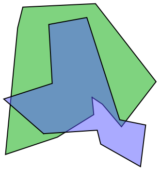
![Module[{rand, p1, p2, bg},
rand = SeedRandom["123"];
p1 = Polygon[RandomInteger[30, {5, 2}]/30];
p2 = Polygon[RandomInteger[30, {5, 2}]/30];
bg = Graphics[{EdgeForm[Thick], Opacity[0],
EdgeForm[Directive[Thick, Red]], p1,
EdgeForm[Directive[Thick, Blue]], p2}];
Map[Show[bg, Graphics[#]] &,
ResourceFunction["PlanarPolygonFragmentation"][p1, p2], {2}]
]](https://www.wolframcloud.com/obj/resourcesystem/images/b75/b75682f5-b29f-4b24-8ecd-41055888a8f4/14ae9ff4f6c48084.png)
![With[{res2 = ResourceFunction["PlanarPolygonFragmentation"][p3, p2]},
Show /@ Map[Graphics[{EdgeForm[Thick], Opacity[.1], #}] &, res2, {2}]
]](https://www.wolframcloud.com/obj/resourcesystem/images/b75/b75682f5-b29f-4b24-8ecd-41055888a8f4/2cd3ae3d86f6ca07.png)

![With[{res2 = ResourceFunction["PlanarPolygonFragmentation"][p3, p2]},
Graphics[{Gray, EdgeForm[Thick],
Apply[ResourceFunction["PlanarPolygonFragmentation"], res2[False][[1 ;; 2]]][True]
}, ImageSize -> 50] // Quiet
]](https://www.wolframcloud.com/obj/resourcesystem/images/b75/b75682f5-b29f-4b24-8ecd-41055888a8f4/3a1c1c0e1456d1ec.png)

![(* Evaluate this cell to get the example input *) CloudGet["https://www.wolframcloud.com/obj/88fd067e-b991-47d2-b67b-3d653e3ced30"]](https://www.wolframcloud.com/obj/resourcesystem/images/b75/b75682f5-b29f-4b24-8ecd-41055888a8f4/463e520f4fd9cf77.png)
![(* Evaluate this cell to get the example input *) CloudGet["https://www.wolframcloud.com/obj/097b92c9-c639-469b-9d56-2a6b807b2dab"]](https://www.wolframcloud.com/obj/resourcesystem/images/b75/b75682f5-b29f-4b24-8ecd-41055888a8f4/73ec1dbae535d047.png)
![(* Evaluate this cell to get the example input *) CloudGet["https://www.wolframcloud.com/obj/4b6a2395-e3e0-4b65-a88d-deb05835d7d6"]](https://www.wolframcloud.com/obj/resourcesystem/images/b75/b75682f5-b29f-4b24-8ecd-41055888a8f4/76817416e6fa3274.png)