Wolfram Function Repository
Instant-use add-on functions for the Wolfram Language
Function Repository Resource:
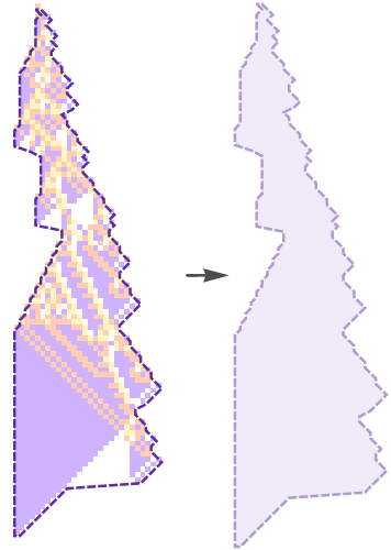
Evolve a cellular automaton with changes to certain cells
ResourceFunction["PerturbedCellularAutomaton"][rule,init,txspec] finds one random location within the body of the automaton and flips the color randomly. | |
ResourceFunction["PerturbedCellularAutomaton"][rule,init,txspec,n] finds n random locations within the body of the automaton and flips the color randomly. | |
ResourceFunction["PerturbedCellularAutomaton"][rule,init,txspec,{tpert,xpert}] flips the cell specified by {tpert, xpert} to a random bit within the number of colors. | |
ResourceFunction["PerturbedCellularAutomaton"][rule,init,txspec,{{tpert1,xpert1}...}] flips all cells in the list of perturbations specifications to a random bit within the number of colors. | |
ResourceFunction["PerturbedCellularAutomaton"][rule,init,txspec,{tpert,xpert}→newbit] flips the cell at indexes specified by {tpert, xpert} to the bit specified by newbit. | |
ResourceFunction["PerturbedCellularAutomaton"][rule,init,txspec,{{tpert1,xpert1}→newbit1...}] flips the cell at indexes {{tpertn, xpertn}...} to bit specified by newbitn. |
| t | perturbs at position t |
| {t1…} | perturbs at position tn in sorted order |
| ts;;te | perturbs at position specified by span in sorted order |
| f | perturbs at indices given by the result running f on the list of possible indices |
| b | sets value of cell to integer b |
| {"AddValue", b} | adds previous value of cell with integer b, modulo the number of colors |
| f | sets value of cell to the result of running f[prev, k] for k colors |
| "Body" | False | whether the indexes given refer to indexes within the body, the body is defined by |
| "ReturnPerturbations" | True | whether to return the performed perturbations, if False, just a list of lists will be returned |
Run a cellular automaton with a random perturbation for 2 steps, here the first cell of the second row is flipped to 0:
| In[1]:= |
| Out[1]= |
Specify that same perturbation:
| In[2]:= |
| Out[2]= |
See the differences based on the perturbation above:
| In[3]:= | ![ArrayPlot /@ {CellularAutomaton[30, {{1}, 0}, {2, {-2, 2}}], First[ResourceFunction[
"PerturbedCellularAutomaton", ResourceSystemBase -> "https://www.wolframcloud.com/obj/resourcesystem/api/1.0"][30, {{1}, 0}, {2, {-2, 2}}, {2, 1} -> 0]]}](https://www.wolframcloud.com/obj/resourcesystem/images/9cd/9cddc4ab-c939-43c9-a92d-685e3d9a055e/2a7b0fde89784f8a.png) |
| Out[3]= |  |
Draw an arrow to the perturbed cell:
| In[4]:= | ![Module[{ca = First[#], pert = Last[#]}, ArrayPlot[ca, Epilog -> {Arrowheads[Large], Style[Arrow[{{0, Length[ca] - #1 - .5}, {#2 - .5 , Length[ca] - #1 - .5}}], Red] & @@@ Keys[pert]}]] &[ ResourceFunction[
"PerturbedCellularAutomaton", ResourceSystemBase -> "https://www.wolframcloud.com/obj/resourcesystem/api/1.0"][30, {{1}, 0}, {2, {-2, 2}}, {2, 1} -> 0]]](https://www.wolframcloud.com/obj/resourcesystem/images/9cd/9cddc4ab-c939-43c9-a92d-685e3d9a055e/128409cf4d364023.png) |
| Out[4]= |  |
Do two random perturbations:
| In[5]:= |
| Out[5]= |
Visualize it:
| In[6]:= | ![Module[{ca = First[#], pert = Last[#]}, ArrayPlot[ca, Epilog -> {Arrowheads[Large], Style[Arrow[{{0, Length[ca] - #1 - .5}, {#2 - .5 , Length[ca] - #1 - .5}}], Red] & @@@ Keys[pert]}]] &[ data]](https://www.wolframcloud.com/obj/resourcesystem/images/9cd/9cddc4ab-c939-43c9-a92d-685e3d9a055e/33968b7eb71aab61.png) |
| Out[6]= | 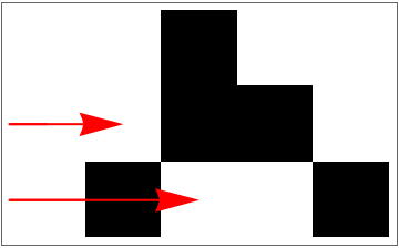 |
Use those same perturbation locations but set them both to white:
| In[7]:= | ![Module[{ca = First[#], pert = Last[#]}, ArrayPlot[ca, Epilog -> {Arrowheads[Large], Style[Arrow[{{0, Length[ca] - #1 - .5}, {#2 - .5 , Length[ca] - #1 - .5}}], Red] & @@@ Keys[pert]}]] &[ ResourceFunction[
"PerturbedCellularAutomaton", ResourceSystemBase -> "https://www.wolframcloud.com/obj/resourcesystem/api/1.0"][
30, {{1}, 0}, {2, {-2, 2}}, {{1, 2}, {2, 4}} -> 0]]](https://www.wolframcloud.com/obj/resourcesystem/images/9cd/9cddc4ab-c939-43c9-a92d-685e3d9a055e/4aa47decb2d2cf46.png) |
| Out[7]= | 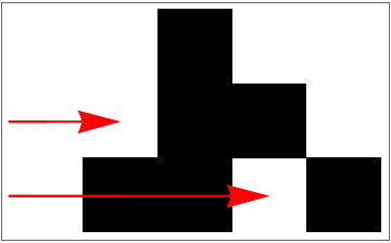 |
Do a range of three perturbations at timestep two:
| In[8]:= |
| Out[8]= |
Visualize it:
| In[9]:= | ![Module[{ca = First[#], pert = Last[#]}, ArrayPlot[ca, Epilog -> {Arrowheads[Large], Style[Arrow[{{0, Length[ca] - #1 - .5}, {#2 - .5 , Length[ca] - #1 - .5}}], Red] & @@@ Keys[pert]}]] &[ data]](https://www.wolframcloud.com/obj/resourcesystem/images/9cd/9cddc4ab-c939-43c9-a92d-685e3d9a055e/7f7961c437591bd3.png) |
| Out[9]= |  |
Perturb the third cell at timestep one and two:
| In[10]:= |
| Out[10]= |
Visualize it:
| In[11]:= | ![Module[{ca = First[#], pert = Last[#]}, ArrayPlot[ca, Epilog -> {Arrowheads[Large], Style[Arrow[{{0, Length[ca] - #1 - .5}, {#2 - .5 , Length[ca] - #1 - .5}}], Red] & @@@ Keys[pert]}]] &[ data]](https://www.wolframcloud.com/obj/resourcesystem/images/9cd/9cddc4ab-c939-43c9-a92d-685e3d9a055e/5e5533e14c37cc70.png) |
| Out[11]= | 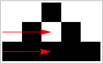 |
Perturb a random sample of three at the second timestep:
| In[12]:= |
| Out[12]= |
Visualize it:
| In[13]:= | ![Module[{ca = First[#], pert = Last[#]}, ArrayPlot[ca, Epilog -> {Arrowheads[Large], Style[Arrow[{{0, Length[ca] - #1 - .5}, {#2 - .5 , Length[ca] - #1 - .5}}], Red] & @@@ Keys[pert]}]] &[ data]](https://www.wolframcloud.com/obj/resourcesystem/images/9cd/9cddc4ab-c939-43c9-a92d-685e3d9a055e/21671b3720ba2adf.png) |
| Out[13]= | 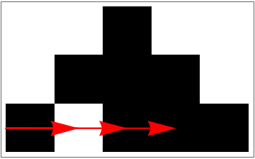 |
Perturb the last cell at every timestep:
| In[14]:= | ![Module[{ca = First[#], pert = Last[#]}, ArrayPlot[ca, Epilog -> {Arrowheads[Large], Style[Arrow[{{0, Length[ca] - #1 - .5}, {#2 - .5 , Length[ca] - #1 - .5}}], Red] & @@@ Keys[pert]}]] &[ ResourceFunction[
"PerturbedCellularAutomaton", ResourceSystemBase -> "https://www.wolframcloud.com/obj/resourcesystem/api/1.0"][30, {{1}, 0}, {2, {-2, 2}}, {;; All, Last}]]](https://www.wolframcloud.com/obj/resourcesystem/images/9cd/9cddc4ab-c939-43c9-a92d-685e3d9a055e/1f52860575f43605.png) |
| Out[14]= | 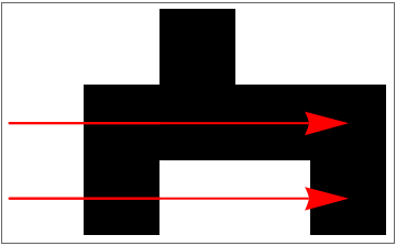 |
With larger k-values, you can use "AddValue" for the bit specification to make a deterministic change. Here yellow always gets flipped to white:
| In[15]:= | ![Module[{ca = First[#], pert = Last[#]}, ArrayPlot[ca, ColorRules -> {0 -> GrayLevel[1], 1 -> Hue[0.06, 1, 1], 2 -> Hue[0.73, 1, 1], 3 -> Hue[0.14, 0.81, 0.99]}, Epilog -> {Arrowheads[Large], Arrow[{{0, Length[ca] - #1 - .5}, {#2 - .5 , Length[ca] - #1 - .5}}] & @@@ Keys[pert]}]] &[
ResourceFunction[
"PerturbedCellularAutomaton", ResourceSystemBase -> "https://www.wolframcloud.com/obj/resourcesystem/api/1.0"][{297413946807002990892857386679107573048, 4, 1}, {{1}, 0}, {30, {-10, 10}}, {{20, 10}, {18, 10}} -> {"AddValue", 1}]]](https://www.wolframcloud.com/obj/resourcesystem/images/9cd/9cddc4ab-c939-43c9-a92d-685e3d9a055e/734e2c0840c7da14.png) |
| Out[15]= | 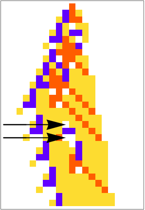 |
Setting "ReturnPerturbations" to False makes it so that only evolution of the automata is returned:
| In[16]:= |
| Out[16]= |
Setting "Body" to true makes it so that the specified index is interpreted as the index within the non-zero range of the automata:
| In[17]:= | ![Module[{ca = First[#], pert = Last[#]}, ArrayPlot[ca, Epilog -> {Arrowheads[Large], Style[Arrow[{{0, Length[ca] - #1 - .5}, {#2 - .5 , Length[ca] - #1 - .5}}], Red] & @@@ Keys[pert]}]] &[ ResourceFunction[
"PerturbedCellularAutomaton", ResourceSystemBase -> "https://www.wolframcloud.com/obj/resourcesystem/api/1.0"][30, {{1}, 0}, {2, {-2, 2}}, {1, 1} -> 0, "Body" -> True]]](https://www.wolframcloud.com/obj/resourcesystem/images/9cd/9cddc4ab-c939-43c9-a92d-685e3d9a055e/47c417cc4e423964.png) |
| Out[17]= |  |
Evolve a rule with perturbations:
| In[18]:= | ![robustru = Module[{ru, ca, lt, pcas, fitness, testcalifetime = Function[ca, If[# == 0, -Infinity, Length[ca] - #] &[
LengthWhile[Reverse[ca], Total[#] == 0 &]]]},
SeedRandom[511114];
Nest[CompoundExpression[
ru = ResourceFunction[
ResourceObject[<|"Name" -> "RandomRuleMutation", "UUID" -> "05a45225-5be5-46bd-9833-9ef3be361333", "ResourceType" -> "Function", "ResourceLocations" -> {
CloudObject[
"https://www.wolframcloud.com/obj/sw-writings0/Resources/05a/05a45225-5be5-46bd-9833-9ef3be361333"]}, "Version" -> None, "DocumentationLink" -> URL[
"https://www.wolframcloud.com/obj/sw-writings0/BiologicalEvolution/RandomRuleMutation"], "ExampleNotebookData" -> Automatic, "FunctionLocation" -> CloudObject[
"https://www.wolframcloud.com/obj/sw-writings0/Resources/05a/05a45225-5be5-46bd-9833-9ef3be361333/download/DefinitionData"], "ShortName" -> "RandomRuleMutation", "SymbolName" -> "FunctionRepository`$05a452255be546bd98339ef3be361333`RandomRuleMutation", "PageHeaderClickToCopy" -> "ResourceObject[CloudObject[\"https://www.wolframcloud.com/obj/sw-writings0/BiologicalEvolution/RandomRuleMutation\"]]"|>]][First[#]],
ca = CellularAutomaton[ru, {{1}, 0}, {200, {-50, 50}}];
lt = testcalifetime[ca];
If[lt == -Infinity, #,
pcas = Table[ResourceFunction[
"PerturbedCellularAutomaton", ResourceSystemBase -> "https://www.wolframcloud.com/obj/resourcesystem/api/1.0"][ru, {{1}, 0}, {200, {-50, 50}}, "ReturnPerturbations" -> False], Ceiling[lt/20]];
fitness = Min[Join[{lt}, testcalifetime /@ pcas]];
If[fitness >= Last[#], {ru, fitness}, #]
]] &, {{0, 4, 1}, 0}, 1000]
] // First;](https://www.wolframcloud.com/obj/resourcesystem/images/9cd/9cddc4ab-c939-43c9-a92d-685e3d9a055e/63518f2a81ebb239.png) |
Plotting our robust automaton:
| In[19]:= | ![ArrayPlot[CellularAutomaton[robustru, {{1}, 0}, {60, {-15, 15}}], ColorRules -> {0 -> GrayLevel[1], 1 -> Hue[0.06, 1, 1], 2 -> Hue[0.73, 1, 1], 3 -> Hue[0.14, 0.81, 0.99]}]](https://www.wolframcloud.com/obj/resourcesystem/images/9cd/9cddc4ab-c939-43c9-a92d-685e3d9a055e/2ef603fa438927e4.png) |
| Out[19]= | 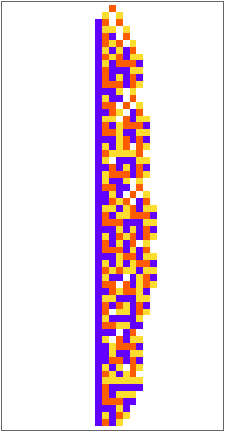 |
Ten sample perturbations:
| In[20]:= | ![Module[{ca = First[#], pert = Last[#]}, ArrayPlot[ca, ColorRules -> {0 -> GrayLevel[1], 1 -> Hue[0.06, 1, 1], 2 -> Hue[0.73, 1, 1], 3 -> Hue[0.14, 0.81, 0.99]}, Epilog -> {Arrowheads[Large], Arrow[{{0, Length[ca] - #1 - .5}, {#2 - .5 , Length[ca] - #1 - .5}}] & @@@ Keys[pert]}]] & /@ Table[ResourceFunction[
"PerturbedCellularAutomaton", ResourceSystemBase -> "https://www.wolframcloud.com/obj/resourcesystem/api/1.0"][robustru, {{1}, 0}, {200, {-20, 20}}], 10]](https://www.wolframcloud.com/obj/resourcesystem/images/9cd/9cddc4ab-c939-43c9-a92d-685e3d9a055e/41575d16ded7d001.png) |
| Out[20]= | 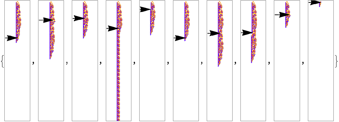 |
Plot the lifetime distribution of one thousand different random single perturbations:
| In[21]:= | ![lts = Function[ca, If[# == 0, 202, Length[ca] - #] &[
LengthWhile[Reverse[ca], Total[#] == 0 &]]] /@ Table[ResourceFunction[
"PerturbedCellularAutomaton", ResourceSystemBase -> "https://www.wolframcloud.com/obj/resourcesystem/api/1.0"][robustru, {{1}, 0}, {200, {-20, 20}}, "ReturnPerturbations" -> False], 1000];
Histogram[lts, PlotRange -> All]](https://www.wolframcloud.com/obj/resourcesystem/images/9cd/9cddc4ab-c939-43c9-a92d-685e3d9a055e/5eef3f05ff7f57fb.png) |
| Out[22]= | 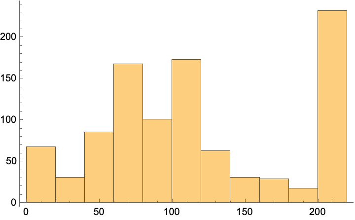 |
Obtain the mortality curve:
| In[23]:= |
| Out[23]= | 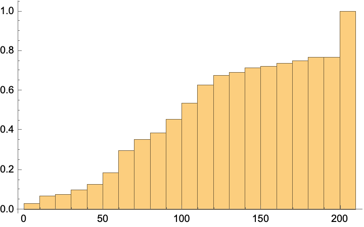 |
When you specify an index outside the range of the body, an empty perturbation is returned:
| In[24]:= |
| Out[24]= |
The tspec uses the same indexing as in CellularAutomaton, so the initial row is perturbed using zero:
| In[25]:= |
| Out[25]= |
Because the automata are stitched together, using All or Automatic as an xspec is not allowed. If no xspec is given, or All or Automatic are given, xspec defaults to {-25,25}:
| In[26]:= | ![ArrayPlot[
First[ResourceFunction[
"PerturbedCellularAutomaton", ResourceSystemBase -> "https://www.wolframcloud.com/obj/resourcesystem/api/1.0"][{297413946807002990892857386679107573048, 4, 1}, {{1}, 0}, 65]], ColorRules -> {0 -> GrayLevel[1], 1 -> Hue[0.06, 1, 1], 2 -> Hue[0.73, 1, 1], 3 -> Hue[0.14, 0.81, 0.99]}]](https://www.wolframcloud.com/obj/resourcesystem/images/9cd/9cddc4ab-c939-43c9-a92d-685e3d9a055e/0df84f226ae06b39.png) |
| Out[26]= | 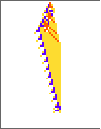 |
Doing many perturbations sometimes results in the body dying out, with no perturbations left to perform:
| In[27]:= | ![Module[{ca = First[#], pert = Last[#]}, ArrayPlot[ca, ColorRules -> {0 -> GrayLevel[1], 1 -> Hue[0.06, 1, 1], 2 -> Hue[0.73, 1, 1], 3 -> Hue[0.14, 0.81, 0.99]}, Epilog -> {Arrowheads[Large], Arrow[{{0, Length[ca] - #1 + .5}, {#2 - .5 , Length[ca] - #1 + .5}}] & @@@ Keys[pert]}]] &[
ResourceFunction[
"PerturbedCellularAutomaton", ResourceSystemBase -> "https://www.wolframcloud.com/obj/resourcesystem/api/1.0"][{180311482541120044137557119353943331376, 4, 1}, {{1}, 0}, {65, {-10, 10}}, 10]]](https://www.wolframcloud.com/obj/resourcesystem/images/9cd/9cddc4ab-c939-43c9-a92d-685e3d9a055e/35afa32a53ab2881.png) |
| Out[27]= |  |
Running the function on an empty list or association returns the unperturbed cellular automaton:
| In[28]:= |
| Out[28]= |
Rules that "age" are particularly robust to perturbations:
| In[29]:= | ![Module[{ca = First[#], pert = Last[#]}, ArrayPlot[ca, ColorRules -> {0 -> GrayLevel[1], 1 -> Hue[0.06, 1, 1], 2 -> Hue[0.73, 1, 1], 3 -> Hue[0.14, 0.81, 0.99]}, Epilog -> {Arrowheads[Large], Arrow[{{0, Length[ca] - #1 + .5}, {#2 - .5 , Length[ca] - #1 + .5}}] & @@@ Keys[pert]}]] &[
ResourceFunction[
"PerturbedCellularAutomaton", ResourceSystemBase -> "https://www.wolframcloud.com/obj/resourcesystem/api/1.0"][{297413946807002990892857386679107573048, 4, 1}, {{1}, 0}, {65, {-10, 10}}]]](https://www.wolframcloud.com/obj/resourcesystem/images/9cd/9cddc4ab-c939-43c9-a92d-685e3d9a055e/1713cc657da94478.png) |
| Out[29]= | 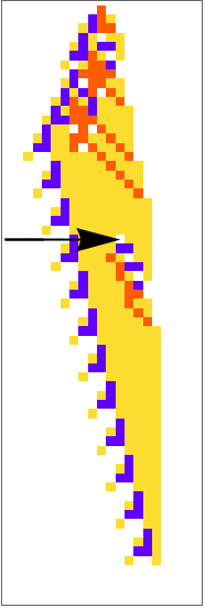 |
They can also be healed easily. Here we apply a therapeutic perturbation:
| In[30]:= | ![Module[{ca = First[#], pert = Last[#]}, ArrayPlot[ca, ColorRules -> {0 -> GrayLevel[1], 1 -> Hue[0.06, 1, 1], 2 -> Hue[0.73, 1, 1], 3 -> Hue[0.14, 0.81, 0.99]}, Epilog -> {Arrowheads[Large], Arrow[{{0, Length[ca] - #1 + .5}, {#2 - .5 , Length[ca] - #1 + .5}}] & @@@ Keys[pert]}]] & /@ (ResourceFunction[
"PerturbedCellularAutomaton", ResourceSystemBase -> "https://www.wolframcloud.com/obj/resourcesystem/api/1.0"][{297413946807002990892857386679107573048, 4, 1}, {{1}, 0}, {65, {-10, 10}}, #] & /@ {{10, 10} -> 3, {{10, 10} -> 3, {15, 8} -> 2}})](https://www.wolframcloud.com/obj/resourcesystem/images/9cd/9cddc4ab-c939-43c9-a92d-685e3d9a055e/274ed2559fba0958.png) |
| Out[30]= | 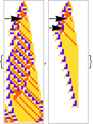 |
With random perturbations you can see the beginning of self-reproduction in very simple rules:
| In[31]:= | ![coords = Transpose@{RandomInteger[{1, 1000}, 500], RandomInteger[{1, 50}, 500]} -> 2;
ArrayPlot[#, ColorRules -> {0 -> GrayLevel[1], 1 -> Hue[0.06, 1, 1], 2 -> Hue[0.73, 1, 1], 3 -> Hue[0.14, 0.81, 0.99]}] &[
ResourceFunction[
"PerturbedCellularAutomaton", ResourceSystemBase -> "https://www.wolframcloud.com/obj/resourcesystem/api/1.0"][{3019941697641, 3, 1}, {{1}, 0}, {{900, 1000}, {-25, 25}}, coords, "ReturnPerturbations" -> False]]](https://www.wolframcloud.com/obj/resourcesystem/images/9cd/9cddc4ab-c939-43c9-a92d-685e3d9a055e/367196dbd0af1905.png) |
| Out[32]= | 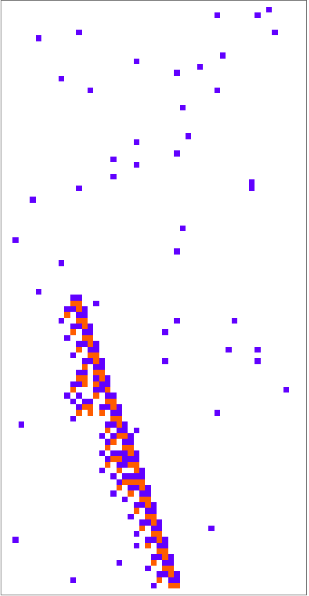 |
Wolfram Language 13.0 (December 2021) or above
This work is licensed under a Creative Commons Attribution 4.0 International License