Wolfram Function Repository
Instant-use add-on functions for the Wolfram Language
Function Repository Resource:
Generate the causal graph produced by combining an unperturbed and perturbed WolframModelEvolutionObject
ResourceFunction["PerturbedCausalGraph"][wm0,wm1] combines the causal graphs of wm0 and wm1 and returns a Graph object. |
Compute a WolframModel evolution over 200 steps:
| In[1]:= | ![wm0 = ResourceFunction[
"WolframModel"][{{{1, 2, 2}, {3, 1, 4}} -> {{2, 5, 2}, {2, 3, 5}, {4, 5, 5}}}, Automatic, 200];
GraphicsRow[{wm0["FinalStatePlot"], wm0["CausalGraph"]}]](https://www.wolframcloud.com/obj/resourcesystem/images/658/658fde6b-d509-4800-a7cb-d074617fbebe/65ec10fe65c95c22.png) |
| Out[2]= | 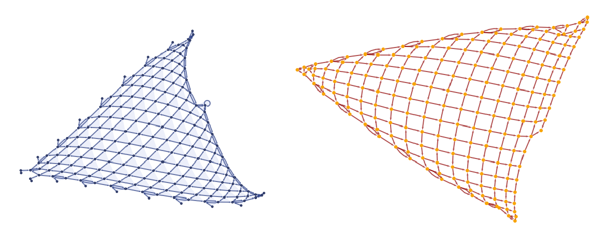 |
After the 200 steps, add a self-loop as a perturbation and evolve for a further 50 steps:
| In[3]:= | ![wm1 = ResourceFunction[
"WolframModel"][{{{1, 2, 2}, {3, 1, 4}} -> {{2, 5, 2}, {2, 3, 5}, {4, 5, 5}}}, Append[wm0["FinalState"], {100, 100, 100}], 50];
GraphicsRow[{wm1["FinalStatePlot"], wm1["CausalGraph"]}]](https://www.wolframcloud.com/obj/resourcesystem/images/658/658fde6b-d509-4800-a7cb-d074617fbebe/6d0f95898ba6af46.png) |
| Out[4]= | 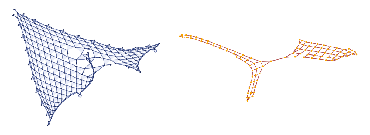 |
Use PerturbedCausalGraph to show the difference caused by the perturbation:
| In[5]:= |
| Out[5]= | 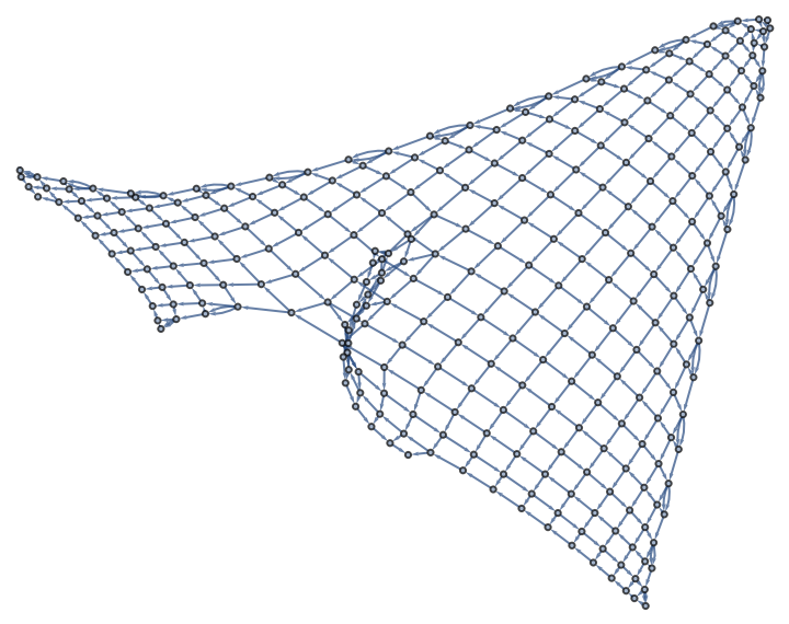 |
Compute 200 steps of the evolution of a WolframModel:
| In[6]:= |
Plot the final state:
| In[7]:= |
| Out[7]= | 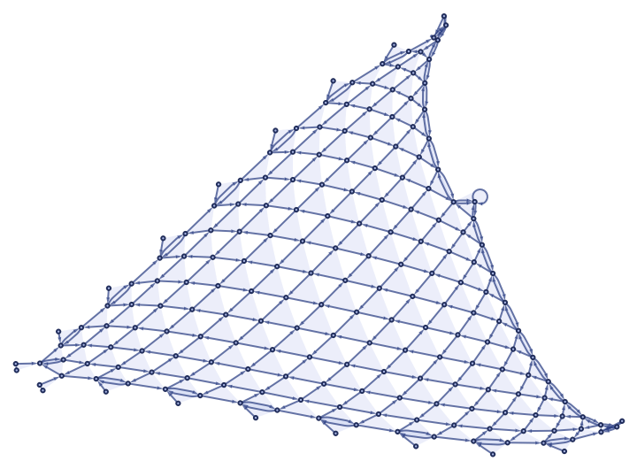 |
Delete 10 random edges in the spatial hypergraph after 200 steps before evolving further:
| In[8]:= | ![wm1 = ResourceFunction[
"WolframModel"][{{{1, 2, 2}, {3, 1, 4}} -> {{2, 5, 2}, {2, 3, 5}, {4, 5, 5}}}, Delete[wm0["FinalState"], Split@RandomSample[Range@Length@wm0["FinalState"], 10]], 200];](https://www.wolframcloud.com/obj/resourcesystem/images/658/658fde6b-d509-4800-a7cb-d074617fbebe/59700465afa632d7.png) |
| In[9]:= |
| Out[9]= | 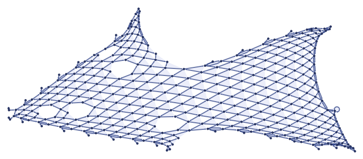 |
Show the perturbed causal graph:
| In[10]:= |
| Out[10]= | 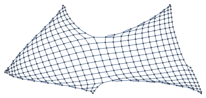 |
Use the output of one rule as the input for a different rule:
| In[11]:= | ![wm0 = ResourceFunction[
"WolframModel"][{{{1, 1, 2}, {2, 3, 4}} -> {{4, 4, 3}, {5, 3, 2}, {2, 5, 1}}}, Automatic, 200];
wm0["CausalGraph"]](https://www.wolframcloud.com/obj/resourcesystem/images/658/658fde6b-d509-4800-a7cb-d074617fbebe/0e6dff0d0007d9e0.png) |
| Out[12]= | 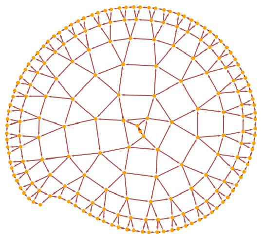 |
| In[13]:= |
| In[14]:= |
| Out[14]= | 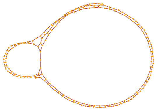 |
| In[15]:= |
| Out[15]= | 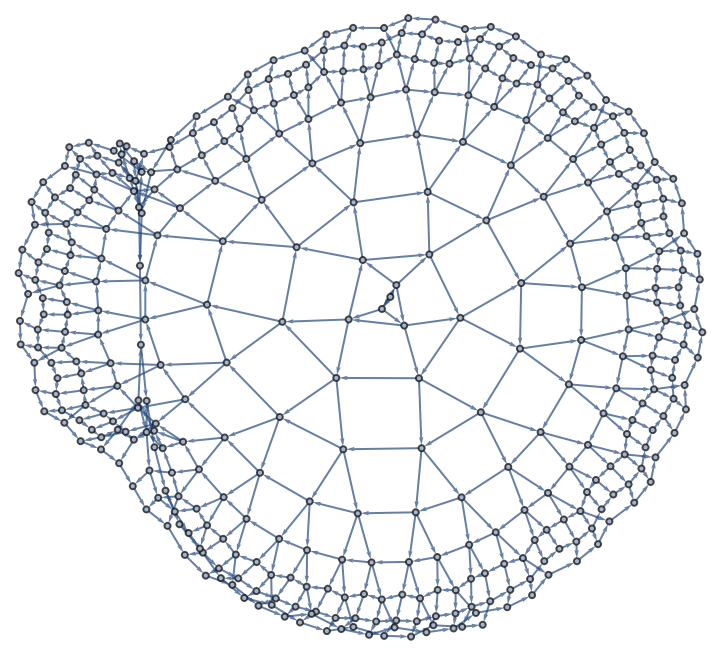 |
This work is licensed under a Creative Commons Attribution 4.0 International License