Basic Examples (2)
Parameterize the line from {0,1} to {1,1} over the domain[0,1]:
Parameterize the 3D polygon formed by three points:
Parameterize the same polygon over the domain[-3,3]:
Evaluate the above parameterization at t=-1/2:
Scope (6)
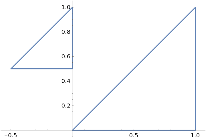
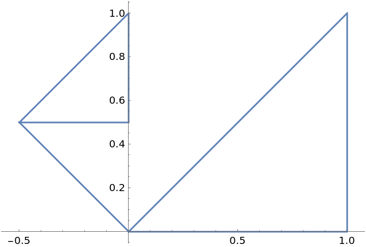
Parameterize a collection of polygons:
Find the linear parameterization between a combination of numeric and symbolic points:
Parameterize a 1D curve:
Parameterize curves in 4 dimensions or greater:
The list of points can be substituted with Rectangle instead:
Substituting with Triangle is also supported:
Besides Triangle[], the heads Line, Triangle, and Polygon are ignored:
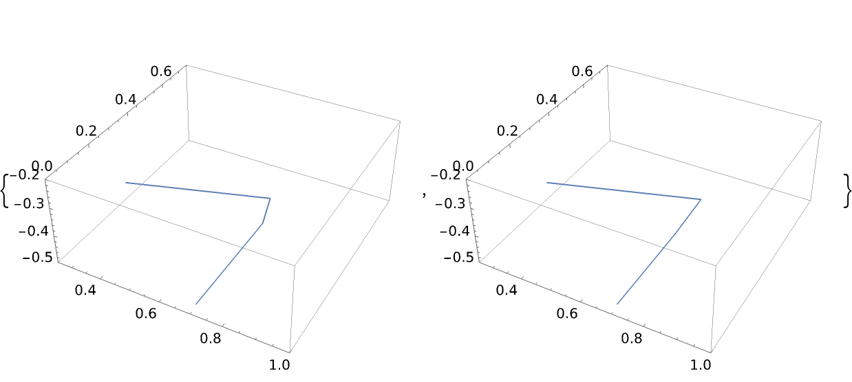
The resulting piecewise function can be input into ParametricPlot or ParametricPlot3D:
Pairs of adjacent points that are the same are treated as a single point:
Options (3)
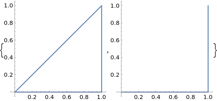
Determine if the list of points defines a closed curve:
Each polygon within a collection is automatically closed:
Setting "ExactValues" to False causes the output to be imprecise:
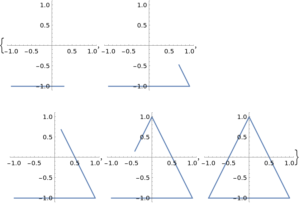
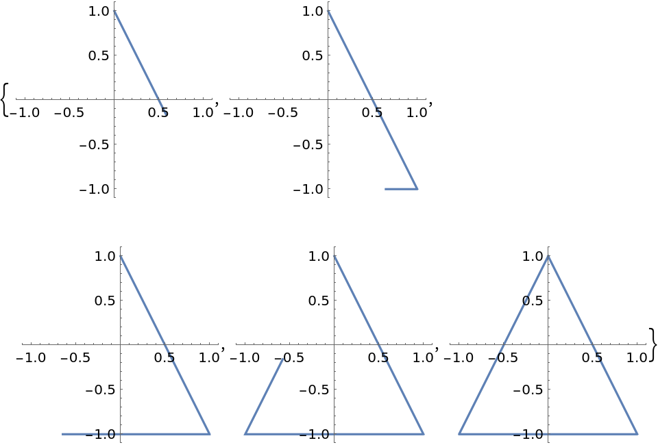
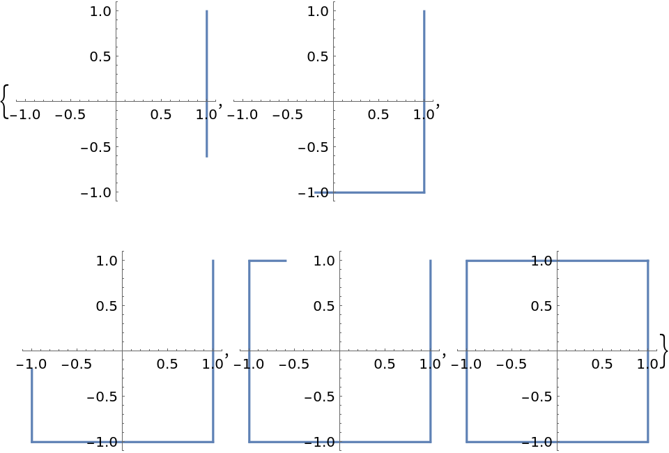
Determine the order of which the points are transversed using the "Orientation" option:
Curves formed using Rectangle are transversed clockwise by default:
The curve formed from Triangle[] is transversed counterclockwise by default:
Applications (5)
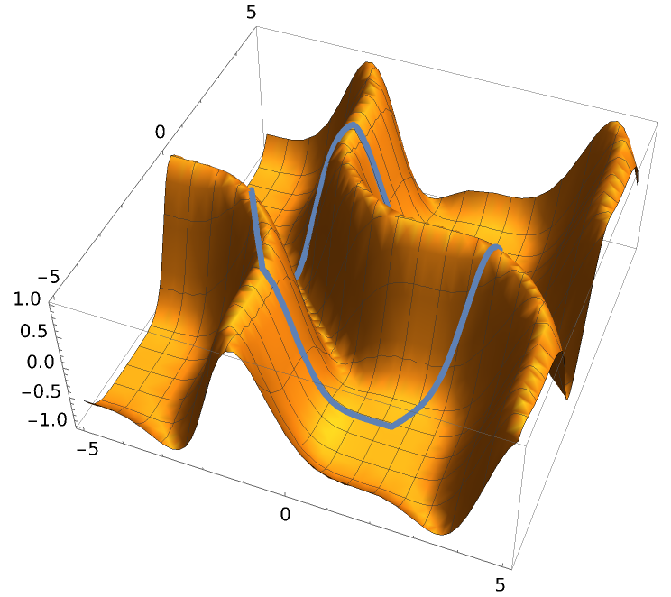
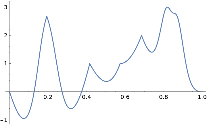
Use the parameterization to analyze a function with 2D domain along a given curve:
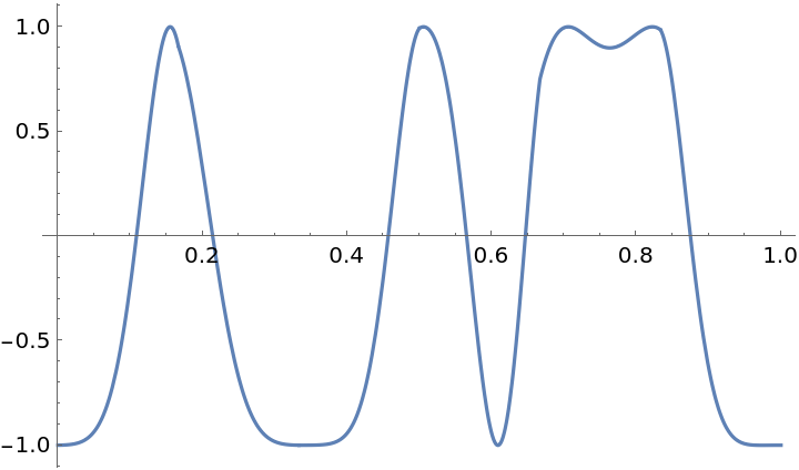
Flatten out the 3D curve to see its output along the parameterization:
Superimpose the output along the parameterization atop the 3D function curve:
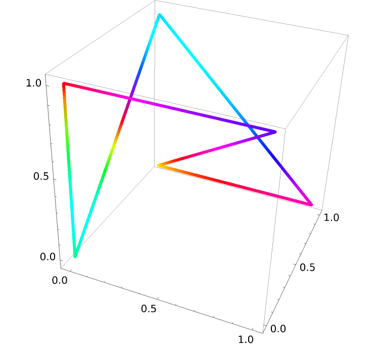
Visualize the output of a function with three variables along a 3D polygon:
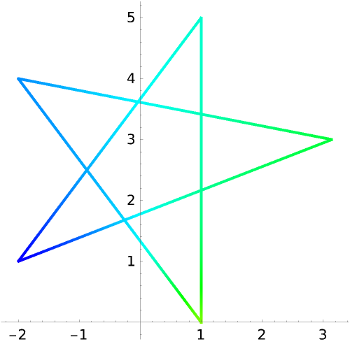
Plot the polygon with Hue shading corresponding to the value of the function:
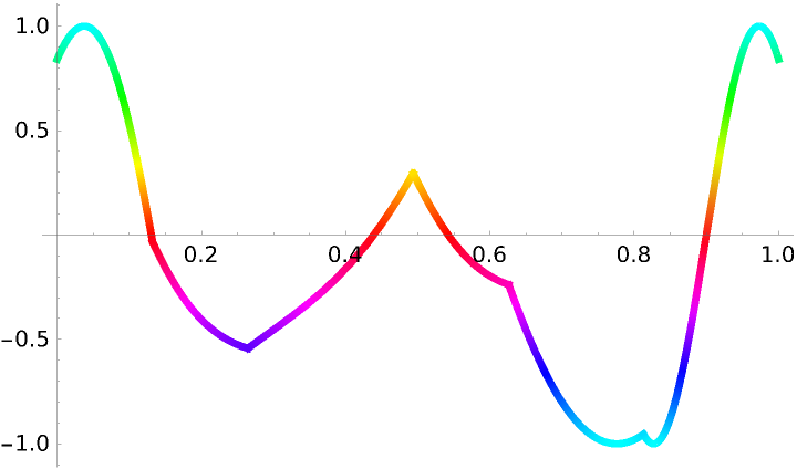
Plot the same function values as a timeline of the parameterization:
This process can be generalized to find the output of a 4 variable function along a 4D curve:
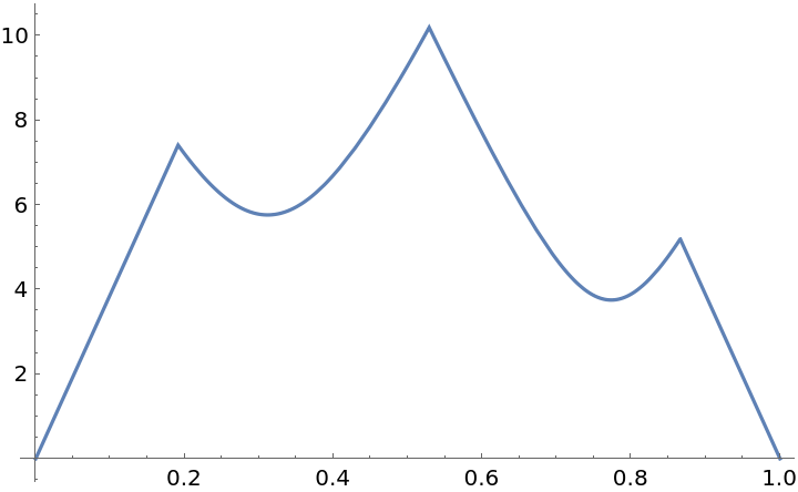
Higher-dimensional polygons can be visualized using Norm along their parameterization:
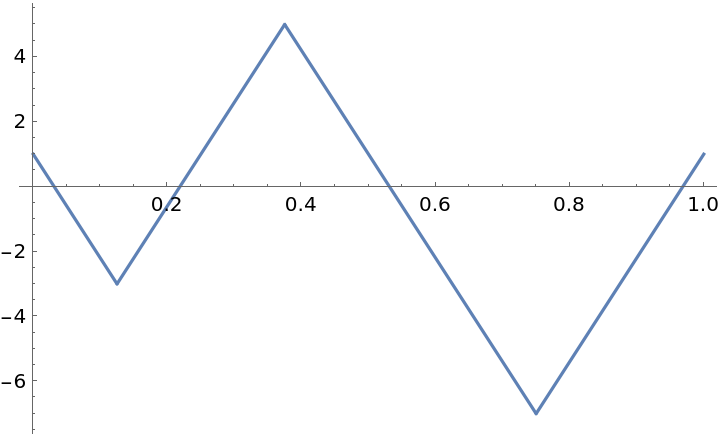
Linear functions can be generated using the plots of 1D polygons:
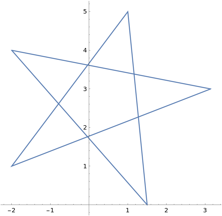
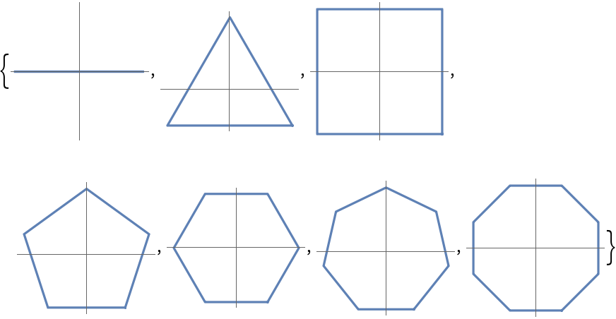
Regular polygons can be parameterized:
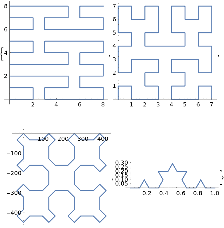
Other named curves can also be parameterized:
Properties and Relations (1)
The resource function ColorWinding uses ParameterizePolygon internally and to generate the "PolygonPlot" output:
Possible Issues (4)
Plotting functions are more efficient when the parameterization has inexact values:
Some polygons encounter a precision error that can be resolved by setting "ExactValues" to False:
Sometimes ParametricPlot will include a connecting line between multiple polygons:
Increasing the number of PlotPoints will remove extraneous points along the curve:
Neat Examples (3)
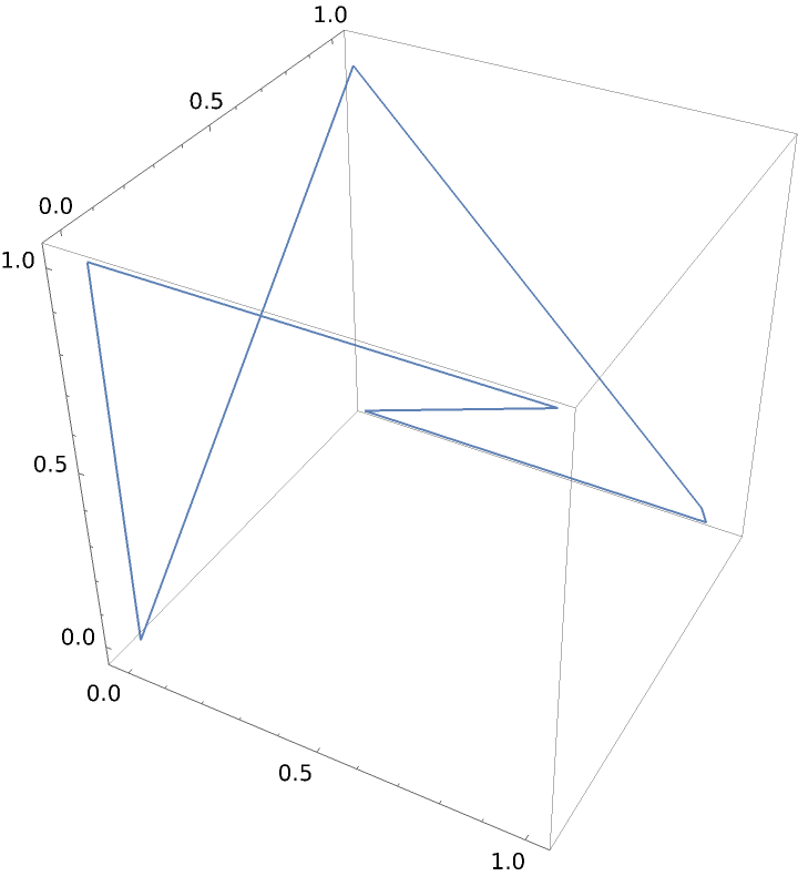
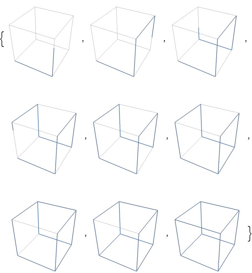
Plot the parameterization of a cube:
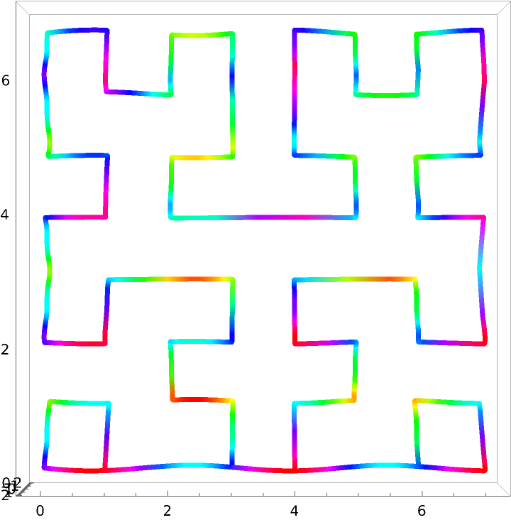
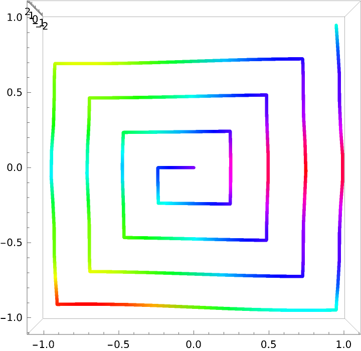
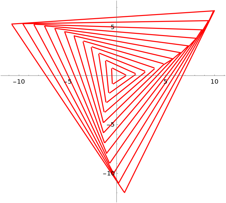
Create abstract shapes using a single parameterization:
Applying a function along a 2D parameterization adds a new dimension to the shape:


![ParametricPlot3D[
ResourceFunction[
"ParameterizePolygon"][{{0, 0, 0}, {0, 0, 1}, {1, 0, 1}, {0, 1, 0}, {1, 1, 0}, {0, 1, 1}}, t], {t, 0, 1}]](https://www.wolframcloud.com/obj/resourcesystem/images/2ce/2ce01e27-52d4-4d6b-a5bb-92ab2648a5d9/2c3fb84984e26cf9.png)
![SameQ[ResourceFunction[
"ParameterizePolygon"][{{0, 0}, {0, 0}, {0, 0}, {1, 1}, {1, 1}}, t],
ResourceFunction["ParameterizePolygon"][{{0, 0}, {1, 1}}, t]]](https://www.wolframcloud.com/obj/resourcesystem/images/2ce/2ce01e27-52d4-4d6b-a5bb-92ab2648a5d9/6d67d84b86838c1d.png)
![ParametricPlot[
ResourceFunction["ParameterizePolygon"][{{0, 0}, {1, 0}, {1, 1}}, t, "ClosedCurve" -> #], {t, 0, 1}] & /@ {True, False}](https://www.wolframcloud.com/obj/resourcesystem/images/2ce/2ce01e27-52d4-4d6b-a5bb-92ab2648a5d9/2f038f29881956ba.png)
![ParametricPlot[
ResourceFunction[
"ParameterizePolygon"][{{{0, 0}, {1, 0}, {1, 1}}, {{-1/2, 1/2}, {0, 1/2}, {0, 1}}}, t], {t, 0, 1}]](https://www.wolframcloud.com/obj/resourcesystem/images/2ce/2ce01e27-52d4-4d6b-a5bb-92ab2648a5d9/0ca33e5c39974e9e.png)

![Table[ParametricPlot[
ResourceFunction["ParameterizePolygon"][{{-1, -1}, {1, -1}, {0, 1}},
t, "Orientation" -> "Forwards"], {t, 0, k}, PlotRange -> 1.1, ImageSize -> 150], {k, 1/5, 1, 1/5}]](https://www.wolframcloud.com/obj/resourcesystem/images/2ce/2ce01e27-52d4-4d6b-a5bb-92ab2648a5d9/170f228116963e7b.png)
![Table[ParametricPlot[
ResourceFunction["ParameterizePolygon"][{{-1, -1}, {1, -1}, {0, 1}},
t, "Orientation" -> "Backwards"], {t, 0, k}, PlotRange -> 1.1, ImageSize -> 150], {k, 1/5, 1, 1/5}]](https://www.wolframcloud.com/obj/resourcesystem/images/2ce/2ce01e27-52d4-4d6b-a5bb-92ab2648a5d9/37843160036de6bf.png)
![Table[ParametricPlot[
ResourceFunction["ParameterizePolygon"][Rectangle[{1, 1}, {-1, -1}],
t], {t, 0, k}, PlotRange -> 1.1, ImageSize -> 150], {k, 1/5, 1, 1/5}]](https://www.wolframcloud.com/obj/resourcesystem/images/2ce/2ce01e27-52d4-4d6b-a5bb-92ab2648a5d9/3ae807da19605a0d.png)
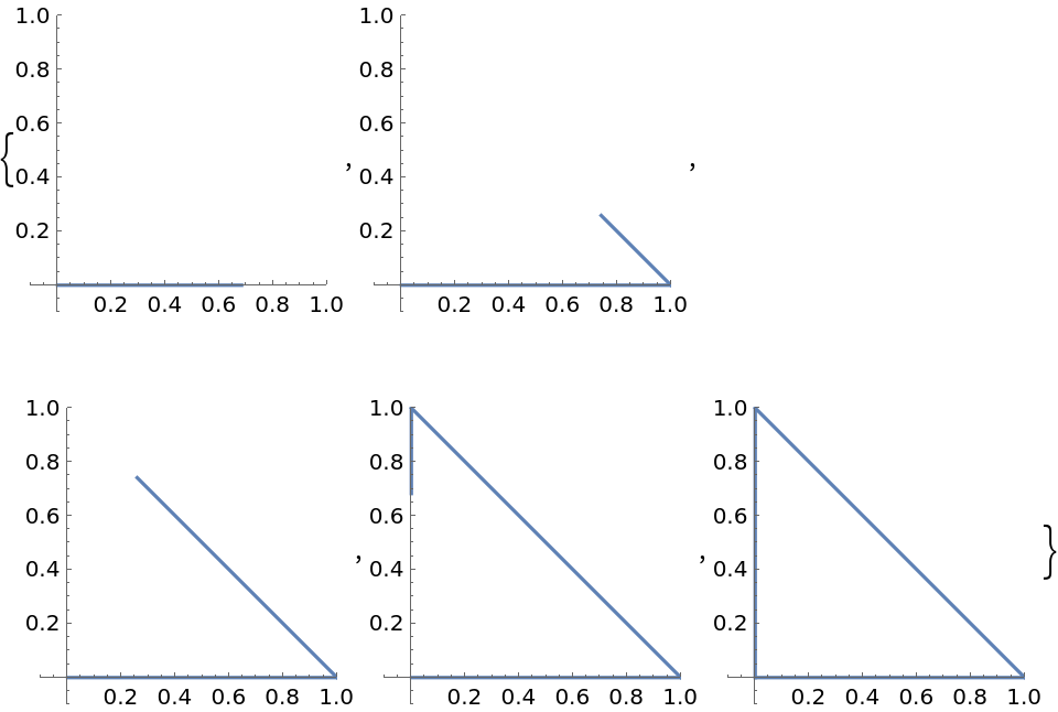
![Table[ParametricPlot[
ResourceFunction["ParameterizePolygon"][Triangle[], t], {t, 0, k}, PlotRange -> {{-0.1, 1}, {-0.1, 1}}, ImageSize -> 150], {k, 1/5, 1, 1/5}]](https://www.wolframcloud.com/obj/resourcesystem/images/2ce/2ce01e27-52d4-4d6b-a5bb-92ab2648a5d9/7ff85b1cf697c405.png)
![paraFun4D[t_] := ResourceFunction[
"ParameterizePolygon"][{{0, 0, 1, 0}, {0, 1, 0, 1}, {1, 0, 1, 0}, {0, 1, 1, 0}, {1, 1, 1, 0}, {1, 0, 1, 1}}, t, "ExactValues" -> False];](https://www.wolframcloud.com/obj/resourcesystem/images/2ce/2ce01e27-52d4-4d6b-a5bb-92ab2648a5d9/4addd1cb78944bed.png)
![Plot[Norm[
ResourceFunction[
"ParameterizePolygon"][{{0, 0, 0, 0, 0}, {1, 2, 3, 4, 5}, {5, -1, 2, 5, -7}, {-1, -4, 1, 0, 3}}, t]], {t, 0, 1}]](https://www.wolframcloud.com/obj/resourcesystem/images/2ce/2ce01e27-52d4-4d6b-a5bb-92ab2648a5d9/69d230f7b2ff7239.png)
![Table[ParametricPlot[
ResourceFunction["ParameterizePolygon"][CirclePoints[k], t, "ExactValues" -> False], {t, 0, 1}, ImageSize -> 100, Ticks -> None], {k, 2, 8}]](https://www.wolframcloud.com/obj/resourcesystem/images/2ce/2ce01e27-52d4-4d6b-a5bb-92ab2648a5d9/695ac5ebffb115d0.png)
![ParametricPlot[
ResourceFunction["ParameterizePolygon"][#, t, "ClosedCurve" -> False, "ExactValues" -> False], {t, 0, 1}] & /@ {PeanoCurve[2], HilbertCurve[3], SierpinskiCurve[2], KochCurve[2]}](https://www.wolframcloud.com/obj/resourcesystem/images/2ce/2ce01e27-52d4-4d6b-a5bb-92ab2648a5d9/2fef78ac87cd2024.png)
![First[AbsoluteTiming[
ParametricPlot3D[
ResourceFunction[
"ParameterizePolygon"][{{0, 0, 0}, {2, 3, 4}, {1, -1, 5}, {5, 9, -12}}, t], {t, 0, 1}]]]](https://www.wolframcloud.com/obj/resourcesystem/images/2ce/2ce01e27-52d4-4d6b-a5bb-92ab2648a5d9/6af21cec438efd64.png)
![First[AbsoluteTiming[
ParametricPlot3D[
ResourceFunction[
"ParameterizePolygon"][{{0, 0, 0}, {2, 3, 4}, {1, -1, 5}, {5, 9, -12}}, t, "ExactValues" -> False], {t, 0, 1}]]]](https://www.wolframcloud.com/obj/resourcesystem/images/2ce/2ce01e27-52d4-4d6b-a5bb-92ab2648a5d9/4882a5fff2722125.png)


![ParametricPlot[
ResourceFunction[
"ParameterizePolygon"][{{{0, 0}, {1, 0}, {1, 1}}, {{-1/2, 1/2}, {0, 1/2}, {0, 1}}}, t, "ExactValues" -> False], {t, 0, 1}]](https://www.wolframcloud.com/obj/resourcesystem/images/2ce/2ce01e27-52d4-4d6b-a5bb-92ab2648a5d9/6756859fea33e95d.png)
![ParametricPlot3D[
ResourceFunction["ParameterizePolygon"][SpherePoints[10], t, "ExactValues" -> False], {t, 0, 1}, ImageSize -> 300, PlotRange -> {{0.25, 1}, {0, .75}, {-.20, -0.5}}, PlotPoints -> #] & /@ {Automatic, {40, 40}}](https://www.wolframcloud.com/obj/resourcesystem/images/2ce/2ce01e27-52d4-4d6b-a5bb-92ab2648a5d9/4a8ee690d0924969.png)
![Table[ParametricPlot3D[
ResourceFunction[
"ParameterizePolygon"][{{0, 0, 0}, {1, 0, 0}, {1, 0, 1}, {1, 1, 1}, {1, 1, 0}, {0, 1, 0}, {0, 1, 1}, {0, 0, 1}, {0, 0, 0}, {1, 0,
0}, {1, 1, 0}, {1, 1, 1}, {0, 1, 1}, {0, 1, 0}, {0, 0, 0}, {0, 0, 1}, {1, 0, 1}, {1, 0, 0}}, t, "ExactValues" -> False], {t, 0, tmax}, PlotPoints -> {300, 300}, ImageSize -> 125, Axes -> False, PlotRange -> {{0, 1}, {0, 1}, {0, 1}}], {tmax, 0.1, 0.9, 0.1}]](https://www.wolframcloud.com/obj/resourcesystem/images/2ce/2ce01e27-52d4-4d6b-a5bb-92ab2648a5d9/06c740e56828fb06.png)
![ParametricPlot[#, {t, 0, 1}, PlotStyle -> Red] &[
ResourceFunction["ParameterizePolygon"][
Table[CirclePoints[k*{1, \[Pi]/64}, 3], {k, 1, 12}], t, "ExactValues" -> False]]](https://www.wolframcloud.com/obj/resourcesystem/images/2ce/2ce01e27-52d4-4d6b-a5bb-92ab2648a5d9/6296e3c3ae5d5dcd.png)
![paraFun3[t_] := ResourceFunction[
"ParameterizePolygon"][{{1, 1}, {1, -1}, {-1, -1}, {-1, 3/4}, {3/4,
3/4}, {3/4, -3/4}, {-3/4, -3/4}, {-3/4, 1/2}, {1/2, 1/2}, {1/2, -1/2}, {-1/2, -1/2}, {-1/2, 1/4}, {1/4, 1/4}, {1/4, -1/4}, {-1/4, -1/4}, {-1/4, 0}, {0, 0}}, t, "ClosedCurve" -> False, "ExactValues" -> False];](https://www.wolframcloud.com/obj/resourcesystem/images/2ce/2ce01e27-52d4-4d6b-a5bb-92ab2648a5d9/750d1574606f8a8c.png)