Wolfram Function Repository
Instant-use add-on functions for the Wolfram Language
Function Repository Resource:
Generate Padua points for bivariate interpolation and cubature
ResourceFunction["PaduaPoints"][n] gives the type 1 Padua points of degree n over the domain [-1,1]×[-1,1]. | |
ResourceFunction["PaduaPoints"][m,n] gives the type m Padua points over the domain [-1,1]×[-1,1]. | |
ResourceFunction["PaduaPoints"][m,n,{{xmin,xmax},{ymin,ymax}}] gives the Padua points over the domain [xmin,xmax]×[ymin,ymax]. | |
ResourceFunction["PaduaPoints"][m,n,{{xmin,xmax},{ymin,ymax}},prec] uses the working precision prec. |
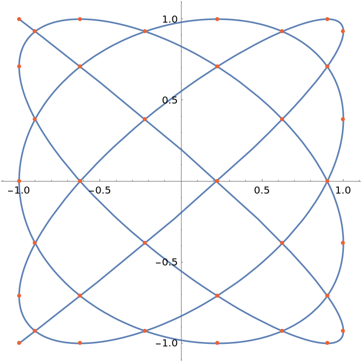
Padua points of degree 3:
| In[1]:= |
|
| Out[1]= |
|
Padua points of type 4 and degree 3:
| In[2]:= |
|
| Out[2]= |
|
Padua points of type 1 and degree 3 over[0,1]×[0,1]:
| In[3]:= |
|
| Out[3]= |
|
Use 25-digit precision:
| In[4]:= |
|
| Out[4]= |

|
A function to approximate:
| In[5]:= |
|
Construct a degree 20 Padua interpolant over[-3,3]×[-3,3]:
| In[6]:= |
|
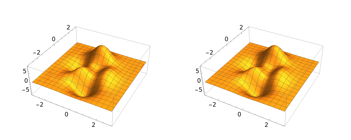
Compare the interpolant with the original function:
| In[7]:= |
|
| Out[7]= |
|
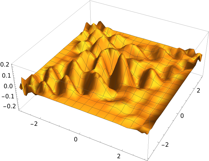
Plot the difference:
| In[8]:= |
|
| Out[8]= |
|
Approximate the integral of a Gaussian function using a degree-25 Padua approximation:
| In[9]:= |
![gau = {x, y} |-> Exp[-x^2 - y^2];
padua = ResourceFunction["PaduaPoints"][1, 25, {{0, 1}, {0, 1}}];
Integrate[
Integrate[
InterpolatingPolynomial[
Transpose[{padua, gau @@@ padua}], {x, y}], {y, 0, 1}], {x, 0, 1}]](https://www.wolframcloud.com/obj/resourcesystem/images/bea/beadb57a-9b1e-4172-8f08-759ff3a4ab64/375ae8f44c3b6332.png)
|
| Out[9]= |
|
Compare with the exact result:
| In[10]:= |
|
| Out[10]= |
|
This work is licensed under a Creative Commons Attribution 4.0 International License
![With[{n = 7},
ParametricPlot[{-Cos[(n + 1) t], -Cos[n t]}, {t, 0, \[Pi]}, Epilog -> {Directive[ColorData[97, 4], AbsolutePointSize[4]], Point[ResourceFunction["PaduaPoints"][n]]}]]](https://www.wolframcloud.com/obj/resourcesystem/images/bea/beadb57a-9b1e-4172-8f08-759ff3a4ab64/26eb20dcfb4196fe.png)